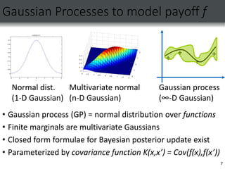
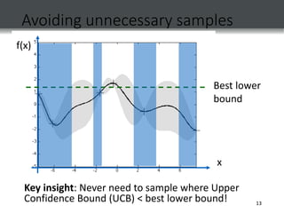
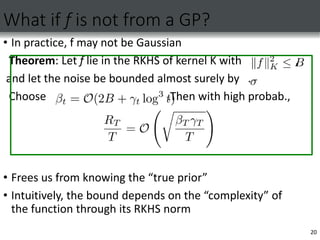
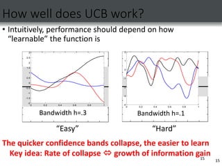
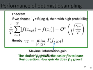
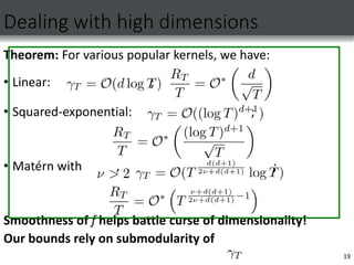
This document discusses Gaussian process bandit optimization, which is a method for adaptively sampling an unknown function to maximize its value. It proposes using an upper confidence bound (UCB) approach, where samples are selected to maximize an upper bound on the function value while also exploring uncertain regions. The key points are: 1) It proves regret bounds for UCB in this setting that depend on how quickly information can be gained about the function from samples, known as the maximal information gain. 2) This connects Gaussian process bandit optimization to Bayesian experimental design, which aims to maximize information gain. 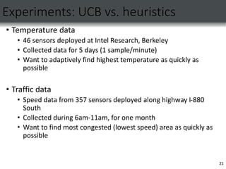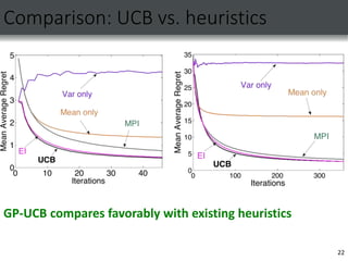3) Experiments on temperature and traffic data show the UCB approach performs comparably to existing heuristics while providing the

1. 1
Multi-armed bandits
• At each time t pick arm i;
• get independent payoff ft with mean ui
• Classic model for exploration – exploitation tradeoff
• Extensively studied (Robbins ’52, Gittins ’79)
• Typically assume each arm is tried multiple times
• Goal: minimize regret
…
u1 u2 u3 uK
1
[ ]
t
T opt t
i
T E f
R 

  

2. 2
Infinite-armed bandits
…
p1 p2 p3 pk
… p∞
p1 p2
…
In many applications, number of arms is huge
(sponsored search, sensor selection)
Cannot try each arm even once
Assumptions on payoff function f essential

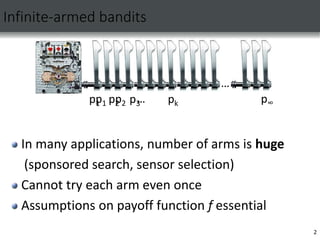
3. Optimizing Noisy, Unknown Functions
• Given: Set of possible inputs D;
black-box access to unknown function f
• Want: Adaptive choice of inputs
from D maximizing
• Many applications: robotic control [Lizotte
et al. ’07], sponsored search [Pande &
Olston, ’07], clinical trials, …
• Sampling is expensive
• Algorithms evaluated using regret
Goal: minimize

4. Running example: Noisy Search
• How to find the hottest point in a building?
• Many noisy sensors available but sampling is expensive
• D: set of sensors; : temperature at chosen at step i
Observe
• Goal: Find with minimal number of queries
4

5. Relating to us: Active learning for PMF
A bandit setting for movie recommendation
Task: recommend movies for a new user
M-armed Bandit
Movie item as arm of bandit
For a new user i
At each round t, pick a movie j
Observe a rating Xij
Goal: maximize cumulative reward
sum of the ratings of all recommended movies
Model: PMF
X=UV+E, where
U: N*K matrix, V: K*M matrix, E: N*M matrix, zero-mean normal distributed
Assume movie feature V is fully observed. User feature Ui is unknown at first
Xi(j) = Ui Vj + ε (regard the ith row vector of X as a function Xi)
Xi(.): random linear function
5

6. Key insight: Exploit correlation
• Sampling f(x) at one point x yields information about f(x’)
for points x’ near x
• In this paper:
Model correlation using a Gaussian process (GP) prior for f
6
Temperature is
spatially correlated

7. Gaussian Processes to model payoff f
• Gaussian process (GP) = normal distribution over functions
• Finite marginals are multivariate Gaussians
• Closed form formulae for Bayesian posterior update exist
• Parameterized by covariance function K(x,x’) = Cov(f(x),f(x’))
7
Normal dist.
(1-D Gaussian)
-2 -1.5 -1 -0.5 0 0.5 1 1.5 2
-2
-1
0
1
2
0
0.1
0.2
0.3
0.4
Multivariate normal
(n-D Gaussian)
+
+
+
+
Gaussian process
(∞-D Gaussian)

8. 8
Thinking about GPs
• Kernel function K(x, x’) specifies covariance
• Encodes smoothness assumptions
x
f(x)
P(f(x))
f(x)

9. 9
Example of GPs
• Squared exponential kernel
K(x,x’) = exp(-(x-x’)2/h2)
0 0.2 0.4 0.6 0.8 1
-4
-3
-2
-1
0
1
2
Bandwidth h=.1
0 100 200 300 400 500 600 700
0
0.1
0.2
0.3
0.4
0.5
0.6
0.7
0.8
0.9
1
Distance |x-x’|
0 0.2 0.4 0.6 0.8 1
-2
-1.5
-1
-0.5
0
0.5
1
1.5
2
2.5
3
Bandwidth h=.3
Samples from P(f)
-3 -2 -1 0 1 2 3

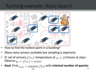
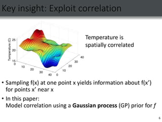
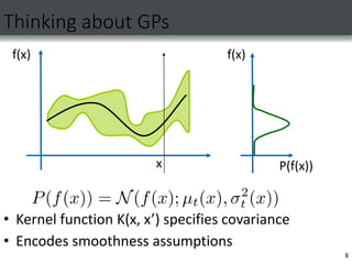
10. Gaussian process optimization
[e.g., Jones et al ’98]
10
x
f(x)
Goal: Adaptively pick
inputs such that
Key question: how should we pick samples?
So far, only heuristics:
Expected Improvement [Močkus et al. ‘78]
Most Probable Improvement [Močkus ‘89]
Used successfully in machine learning [Ginsbourger et al. ‘08,
Jones ‘01, Lizotte et al. ’07]
No theoretical guarantees on their regret!

11. 11
Simple algorithm for GP optimization
• In each round t do:
• Pick
• Observe
• Use Bayes’ rule to get posterior mean
Can get stuck in local maxima!
11
x
f(x)

12. 12
Uncertainty sampling
Pick:
That’s equivalent to (greedily) maximizing
information gain
Popular objective in Bayesian experimental design
(where the goal is pure exploration of f)
But…wastes samples by exploring f everywhere!
12
x
f(x)

13. Avoiding unnecessary samples
Key insight: Never need to sample where Upper
Confidence Bound (UCB) < best lower bound! 13
x
f(x)
Best lower
bound

14. 14
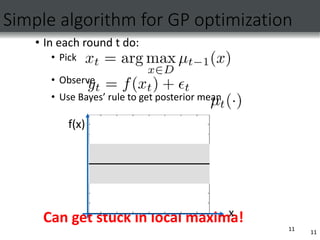
Upper Confidence Bound (UCB) Algorithm
Naturally trades off explore and exploit; no samples wasted
Regret bounds: classic [Auer ’02] & linear f [Dani et al. ‘07]
But none in the GP optimization setting! (popular heuristic)
x
f(x)
Pick input that maximizes Upper Confidence Bound (UCB):
How should
we choose ¯t?
Need theory!

15. 15
How well does UCB work?
• Intuitively, performance should depend on how
“learnable” the function is
15
“Easy” “Hard”
The quicker confidence bands collapse, the easier to learn
Key idea: Rate of collapse  growth of information gain
0 0.2 0.4 0.6 0.8 1
-2
-1.5
-1
-0.5
0
0.5
1
1.5
2
2.5
3
Bandwidth h=.3
0 0.2 0.4 0.6 0.8 1
-4
-3
-2
-1
0
1
2
Bandwidth h=.1

16. Learnability and information gain
• We show that regret bounds depend on how quickly we can
gain information
• Mathematically:
• Establishes a novel connection between GP optimization
and Bayesian experimental design
16
T

17. 17
Performance of optimistic sampling
Theorem
If we choose ¯t = £(log t), then with high probability,
Hereby
The slower γT grows, the easier f is to learn
Key question: How quickly does γ T grow?
17
Maximal information gain
due to sampling!

18. Learnability and information gain
• Information gain exhibits diminishing returns (submodularity)
[Krause & Guestrin ’05]
• Our bounds depend on “rate” of diminishment
18
Little diminishing returns
Returns diminish fast

19. Dealing with high dimensions
Theorem: For various popular kernels, we have:
• Linear: ;
• Squared-exponential: ;
• Matérn with , ;
Smoothness of f helps battle curse of dimensionality!
Our bounds rely on submodularity of
19

20. What if f is not from a GP?
• In practice, f may not be Gaussian
Theorem: Let f lie in the RKHS of kernel K with ,
and let the noise be bounded almost surely by .
Choose .Then with high probab.,
• Frees us from knowing the “true prior”
• Intuitively, the bound depends on the “complexity” of
the function through its RKHS norm
20

21. Experiments: UCB vs. heuristics
• Temperature data
• 46 sensors deployed at Intel Research, Berkeley
• Collected data for 5 days (1 sample/minute)
• Want to adaptively find highest temperature as quickly as
possible
• Traffic data
• Speed data from 357 sensors deployed along highway I-880
South
• Collected during 6am-11am, for one month
• Want to find most congested (lowest speed) area as quickly as
possible
21

22. Comparison: UCB vs. heuristics
22
GP-UCB compares favorably with existing heuristics

23. 23
Assumptions on f
Linear?
[Dani et al, ’07]
Lipschitz-continuous
(bounded slope)
[Kleinberg ‘08]
Fast convergence;
But strong assumption
Very flexible, but

24. Conclusions
• First theoretical guarantees and convergence rates
for GP optimization
• Both true prior and agnostic case covered
• Performance depends on “learnability”, captured by
maximal information gain
• Connects GP Bandit Optimization & Experimental Design!
• Performance on real data comparable to other heuristics
24