
![Background - Genetic Programming
• [Nichael L. Cramer - 1985]
• [John R. Koza - 1992]
• evolutionary-based search strategy
• dynamic and tree-structure representation
• favors the use of programming language that naturally embody tree structure](https://image.slidesharecdn.com/gp-130129140247-phpapp01/85/Genetic-programming-3-320.jpg)
![The problem with recursion (1/3)
• infinite loop in strict evaluation
• finite limit on recursive calls [Brave - 1996]
• finite limit on execution time [Wong & Leung - 1996]
• the “Map” function [Clack & Yu - 1997]
• “Map”, a higher-order function, can work on a finite list
• a non-terminated program with good properties
may or may not be discarded in selection step](https://image.slidesharecdn.com/gp-130129140247-phpapp01/85/Genetic-programming-6-320.jpg)
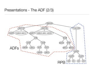
![Presentations - The ADF (1/3)
• Automatically Defined Function (ADF) [Koza - 1994]
• Divide and Conquer:
• each program in population contains two main parts:
i. result-producing branch (RPB)
ii.definition of one or more functions (ADFs)](https://image.slidesharecdn.com/gp-130129140247-phpapp01/85/Genetic-programming-9-320.jpg)
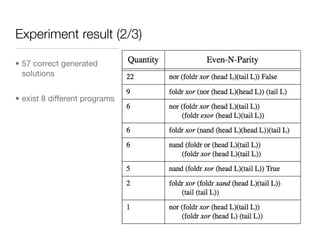
![The experiment (1/2)
• Even-N-Parity problem
• has been used as a difficult problem for GP [Koza - 1992]
• returning True if an even number of input are true
• Function Set {AND, OR, NAND, NOR}
• Terminal Set {b0, b1, ..., bN-1} with N boolean variables
• testing instance consists of all the binary strings with length N
[00110100] → 3 → False
[01100101] → 4 → True](https://image.slidesharecdn.com/gp-130129140247-phpapp01/85/Genetic-programming-13-320.jpg)
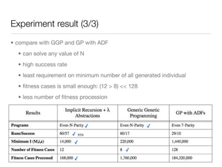
![The experiment (2/2)
• using GP only [Koza - 1992]
• can solve the problem with very high accuracy when 1 ≤ N ≤ 5
• using GP with ADF [Koza - 1994]
• can solve this problem up to N = 11
• using GP with a logic grammar [Wong & Leung - 1996]
• according to the Curry-Howard Isomorphism, a logic system consists a
type system that can describe some semantics
• strong enough to handle any value of N
• however, any noisy case will increase the computational cost](https://image.slidesharecdn.com/gp-130129140247-phpapp01/85/Genetic-programming-14-320.jpg)
![Type system (1/4)
• using type system to reserve the structure of program
• for example: in even-n-parity, program :: [Bool] → Bool
• we can also using type system to run GP with slight semantics
• perform type checking during crossover and mutation
• to ensure the resulting program is reasonable](https://image.slidesharecdn.com/gp-130129140247-phpapp01/85/Genetic-programming-19-320.jpg)
![Type system (4/4)
• foldr :: (a→b→b) →b →[a] →b
• glue function (induction) (a→b→b) →b →[a] →b
• base case (a→b→b) →b →[a] →b
• foldr takes two arguments and return a function
that takes a list of some type a and return a single value with type b
• example: foldr (+) 0 [1,2,3] = foldr (+) 0 (1:(2:(3:[ ]))) = (1+(2+(3+0))) = 6
• another example: foldr xor F [T,F] = (xor T (xor F F)) = (xor T F) = T
• another example: foldr (λ.λ.and T P1) T [1,2] = ((λ.λ.and T P1) 1 ((λ.λ.and T P1)
2 ((λ.λ.and T P1) T))) = ((λ.λ.and T P1) 1 ((λ.λ.and T P1) 2 T)) = ((λ.λ.and T P1) 1
T) = and T T = T](https://image.slidesharecdn.com/gp-130129140247-phpapp01/85/Genetic-programming-22-320.jpg)
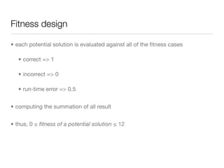
![Experimentation
• maximum depth of nested recursion = 100
• simple example with depth = 2
foldr
+ [1,2,3]
foldr
+ [1,2,3]
0](https://image.slidesharecdn.com/gp-130129140247-phpapp01/85/Genetic-programming-24-320.jpg)

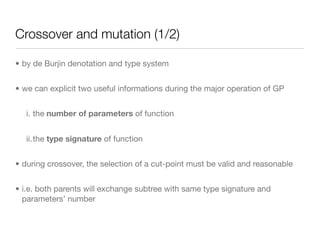
![Selection of cut-point
• because of the using of fold and λ abstract, a node with a less depth will have
a stronger description:
foldr
+ [1,2,3]
foldr
+ [1,2,3]
0
• adopting a method: node have a higher chance to be selected by crossover if
it is more close root](https://image.slidesharecdn.com/gp-130129140247-phpapp01/85/Genetic-programming-27-320.jpg)
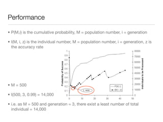

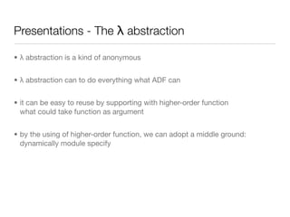
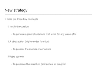
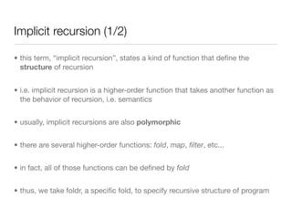
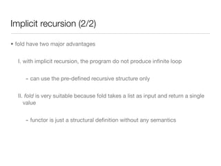
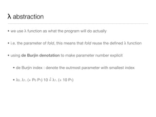
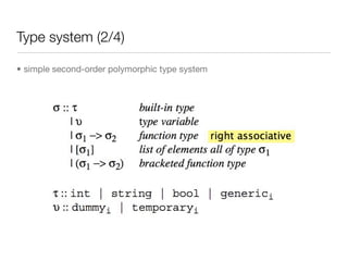
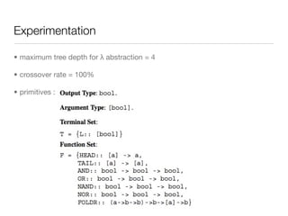
The document discusses using genetic programming with lambda abstractions and recursion to solve problems like parity. It outlines challenges with recursion in genetic programming like infinite loops. A new strategy is proposed using implicit recursion with higher-order functions like fold, lambda abstractions to define program structure, and a type system to preserve semantics. An experiment applies this approach to the even-n-parity problem, generating programs that work for any input size with high success rates using fewer individuals than other methods.