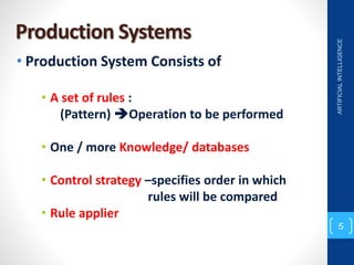
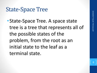
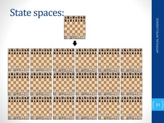
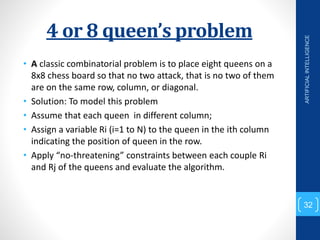
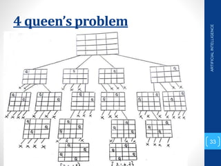
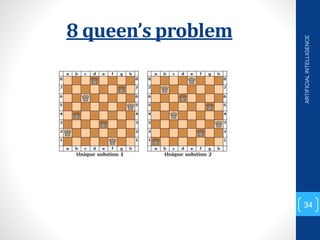
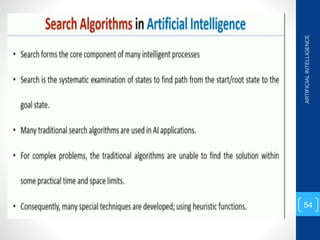
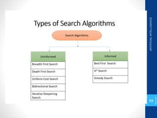
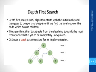
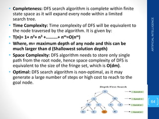
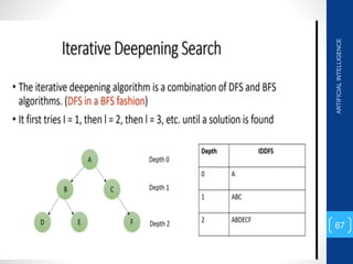
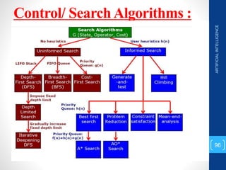
Module_2_rks in Artificial intelligence in Expert System

MODULE 2
Problem Solving Agents – Searching for
solutions- Uninformed Search Strategies
– Informed Search Strategies, heuristic
functions.

Artificial intelligence
• Intelligence : “Ability to learn, understand,
and think”.
• The study of the capacity of machines to
simulate intelligent human behavior.
• AI is the study of how to make computers
make things which at the moment people
do better.
ARTIFICIAL
INTELLIGENCE
2

Problem solving System
•Define the problem.
•Analyze the problem.
•Isolate & represent the task
knowledge necessary to solve the
problem.
•Choose the best problem- solving
techniques & apply it to the problem.
ARTIFICIAL
INTELLIGENCE
3

Formal description for defining
a problem
•Representation :
•State Space
• It contains set of all the possible states of
the relevant problem
•Initial State
•Goal State
•Transformation Rules
ARTIFICIAL
INTELLIGENCE
4

Production Systems
• Production System Consists of
• A set of rules :
(Pattern) Operation to be performed
• One / more Knowledge/ databases
• Control strategy –specifies order in which
rules will be compared
• Rule applier
ARTIFICIAL
INTELLIGENCE
5

State-Space Tree
•State-Space Tree. A space state
tree is a tree that represents all of
the possible states of the
problem, from the root as an
initial state to the leaf as a
terminal state.
ARTIFICIAL
INTELLIGENCE
6

• Let G= (V,E) be a directed graph with each edge cost cij.
• Cij is defined such that cij.>0 for all I and j and cij = ∞ if (i,j) not
belongs to E.
• A tour of G is a directed simple cycle that includes every
vertex in V.
• The cost of a tour is the sum of the cost of edges on the tour.
The TVs problem is to find a tour of minimum cost.
• For example: consider a production environment in wchich
several commodities are manufactured by same set of
machines. The manufacture proceeds in cycles. In each
production cycle, n different commodities are produced.
When the machines are changed from production of
commodity I to commodity j, a change over cost cij is incurred.
ARTIFICIAL
INTELLIGENCE
17

Tower of Hanoi
ARTIFICIAL
INTELLIGENCE
19

Tower of Hanoi
ARTIFICIAL
INTELLIGENCE
20

Tower of Hanoi
ARTIFICIAL
INTELLIGENCE
21

Chess board- problem
• Defining the problem as a state space search:
• Start the problem of play chess.
• 1st we have to specify the starting position of chess board, the
rules that define the legal moves, and the board positions that
represent a win for one side or the other.
• Problem description:
• Consider a chess board 8x8 array where each position
contains a symbol standing for the appropriate piece in
the official chess opening position
ARTIFICIAL
INTELLIGENCE
26

Chess board- problem
• Goal state:
• The goal of any board in which the opponent does not have a
legal move and his or her king is under attack.
• Legal move from initial state to final state.
• If we write legal moves of roughly 10120 possible board
positions.
ARTIFICIAL
INTELLIGENCE
27

Game Playing
ARTIFICIAL
INTELLIGENCE
28

Game Playing
ARTIFICIAL
INTELLIGENCE
29

Chess game
ARTIFICIAL
INTELLIGENCE
30
Transformation Rules:
white pawn at
square(file e, rank 2)
AND
square(file e, rank 3) is empty
AND
square(file e, rank 4) is empty
Initial state: Current board position Goal state: opponent does not have a
legal move and his /her king is under
attack.
Move pawn from
to

State spaces:
ARTIFICIAL
INTELLIGENCE
31

4 or 8 queen’s problem
• A classic combinatorial problem is to place eight queens on a
8x8 chess board so that no two attack, that is no two of them
are on the same row, column, or diagonal.
• Solution: To model this problem
• Assume that each queen in different column;
• Assign a variable Ri (i=1 to N) to the queen in the ith column
indicating the position of queen in the row.
• Apply “no-threatening” constraints between each couple Ri
and Rj of the queens and evaluate the algorithm.
ARTIFICIAL
INTELLIGENCE
32

4 queen’s problem
ARTIFICIAL
INTELLIGENCE
33

8 queen’s problem
ARTIFICIAL
INTELLIGENCE
34

• Time Complexity: Time Complexity of BFS algorithm can be
obtained by the number of nodes traversed in BFS until the
shallowest Node. Where the d= depth of shallowest solution
and b is a node at every state.
• T (b) = 1+b2+b3+.......+ bd= O (bd)
• Space Complexity: Space complexity of BFS algorithm is given
by the Memory size of frontier which is O(bd).
• Completeness: BFS is complete, which means if the shallowest
goal node is at some finite depth, then BFS will find a solution.
• Optimality: BFS is optimal if path cost is a non-decreasing
function of the depth of the node
ARTIFICIAL
INTELLIGENCE
62

• Completeness: DFS search algorithm is complete within finite
state space as it will expand every node within a limited
search tree.
• Time Complexity: Time complexity of DFS will be equivalent to
the node traversed by the algorithm. It is given by:
• T(n)= 1+ n2+ n3 +.........+ nm=O(nm)
• Where, m= maximum depth of any node and this can be
much larger than d (Shallowest solution depth)
• Space Complexity: DFS algorithm needs to store only single
path from the root node, hence space complexity of DFS is
equivalent to the size of the fringe set, which is O(dm).
• Optimal: DFS search algorithm is non-optimal, as it may
generate a large number of steps or high cost to reach to the
goal node.
ARTIFICIAL
INTELLIGENCE
64

• Completeness:
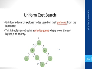
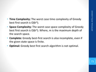
• Uniform-cost search is complete, such as if there is a solution, UCS
will find it.
• Time Complexity:
• Let C* is Cost of the optimal solution, and ε is each step to get
closer to the goal node. Then the number of steps is = C*/ε. Here we
have taken +1, as we start from state 0 and end to C*/ε.
• Hence, the worst-case time complexity of Uniform-cost search
isO(b1 + [C*/ε])/.
• Space Complexity:
• The same logic is for space complexity so, the worst-case space
complexity of Uniform-cost search is O(b1 + [C*/ε]).
• Optimal:
• Uniform-cost search is always optimal as it only selects a path with
the lowest path cost.
ARTIFICIAL
INTELLIGENCE
66

• Completeness:
• This algorithm is complete is if the branching factor is finite.
• Time Complexity:
• Let's suppose b is the branching factor and depth is d then the
worst-case time complexity is O(bd).
• Space Complexity:
• The space complexity of IDDFS will be O(bd).
• Optimal:
• IDDFS algorithm is optimal if path cost is a non- decreasing
function of the depth of the node.
ARTIFICIAL
INTELLIGENCE
68

• Completeness: Bidirectional Search is complete if we use BFS
in both searches.
• Time Complexity: Time complexity of bidirectional search
using BFS is O(bd).
• Space Complexity: Space complexity of bidirectional search
is O(bd).
• Optimal: Bidirectional search is Optimal
ARTIFICIAL
INTELLIGENCE
70

• Time Complexity: The worst case time complexity of Greedy
best first search is O(bm).
• Space Complexity: The worst case space complexity of Greedy
best first search is O(bm). Where, m is the maximum depth of
the search space.
• Complete: Greedy best-first search is also incomplete, even if
the given state space is finite.
• Optimal: Greedy best first search algorithm is not optimal.
ARTIFICIAL
INTELLIGENCE
73

• Time Complexity: The worst case time complexity of Greedy
best first search is O(bm).
• Space Complexity: The worst case space complexity of Greedy
best first search is O(bm). Where, m is the maximum depth of
the search space.
• Complete: Greedy best-first search is also incomplete, even if
the given state space is finite.
• Optimal: Greedy best first search algorithm is not optimal.
ARTIFICIAL
INTELLIGENCE
85

Control/ SearchAlgorithms :
ARTIFICIAL
INTELLIGENCE
96

Module_2_rks in Artificial intelligence in Expert System

More Related Content

Similar to Module_2_rks in Artificial intelligence in Expert System

Recently uploaded

Module_2_rks in Artificial intelligence in Expert System