Download as PDF, PPTX


![The ADWIN Algorithm - Notations and Settings
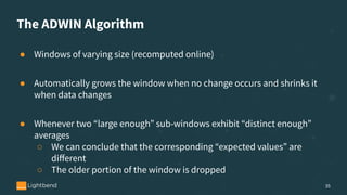
• a (possibly infinite) sequence of real values x1
, x2
, .. , xt
, ..
• a confidence value 𝛿 ∈ (0, 1)
• the value of xt
is available only at time t
• each xt
is generated according to some distribution Dt
independent of every t
• 𝜇t
and 𝜎t
2
denote the expected value and variance of xt
when it is drawn according to Dt
• xt
is always in [0, 1]
36](https://image.slidesharecdn.com/onlinemachinelearning-191004194829/85/Online-machine-learning-in-Streaming-Applications-36-320.jpg)


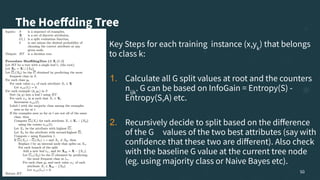


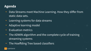
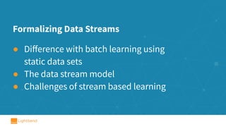
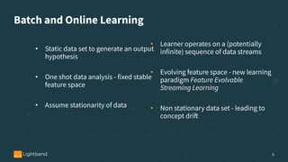
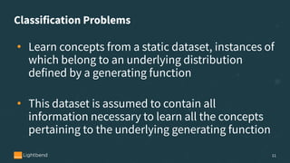
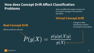
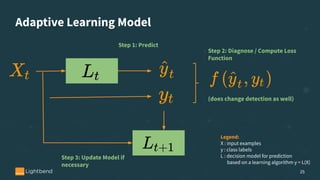
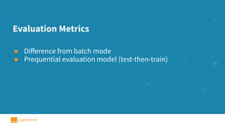
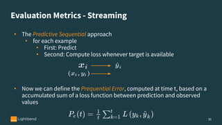
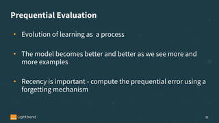
The document discusses online machine learning in streaming applications, emphasizing the differences between data streams and static datasets, as well as the challenges of stream-based learning, such as concept drift and evolving feature spaces. It covers learning systems' desirable properties, evaluation metrics, and specific algorithms like the Adwin algorithm and Hoeffding tree classifiers for handling real-time data. The presentation highlights the adaptive learning model necessary for processing continuous data while managing memory constraints and adapting to changes in data distribution.