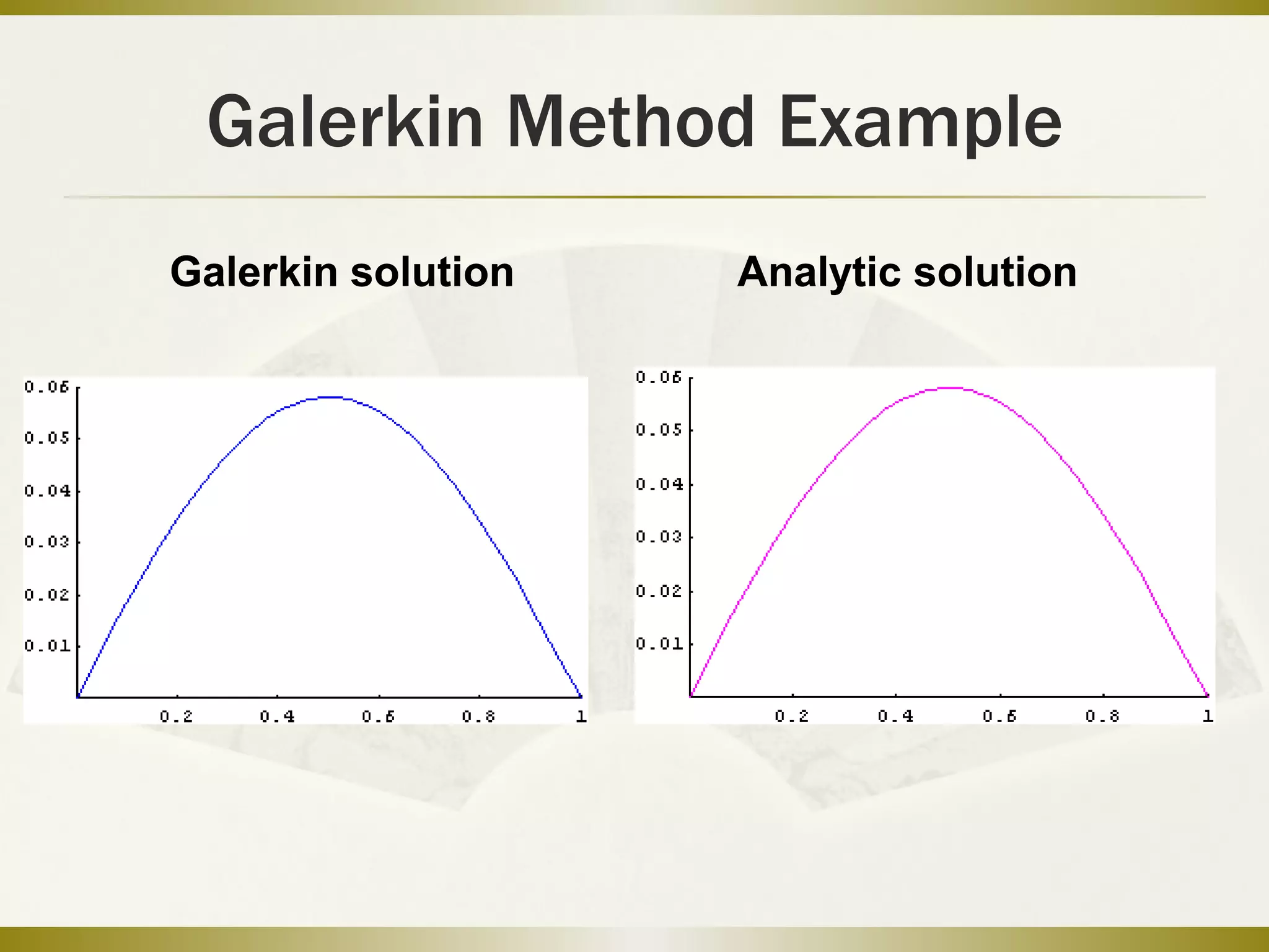
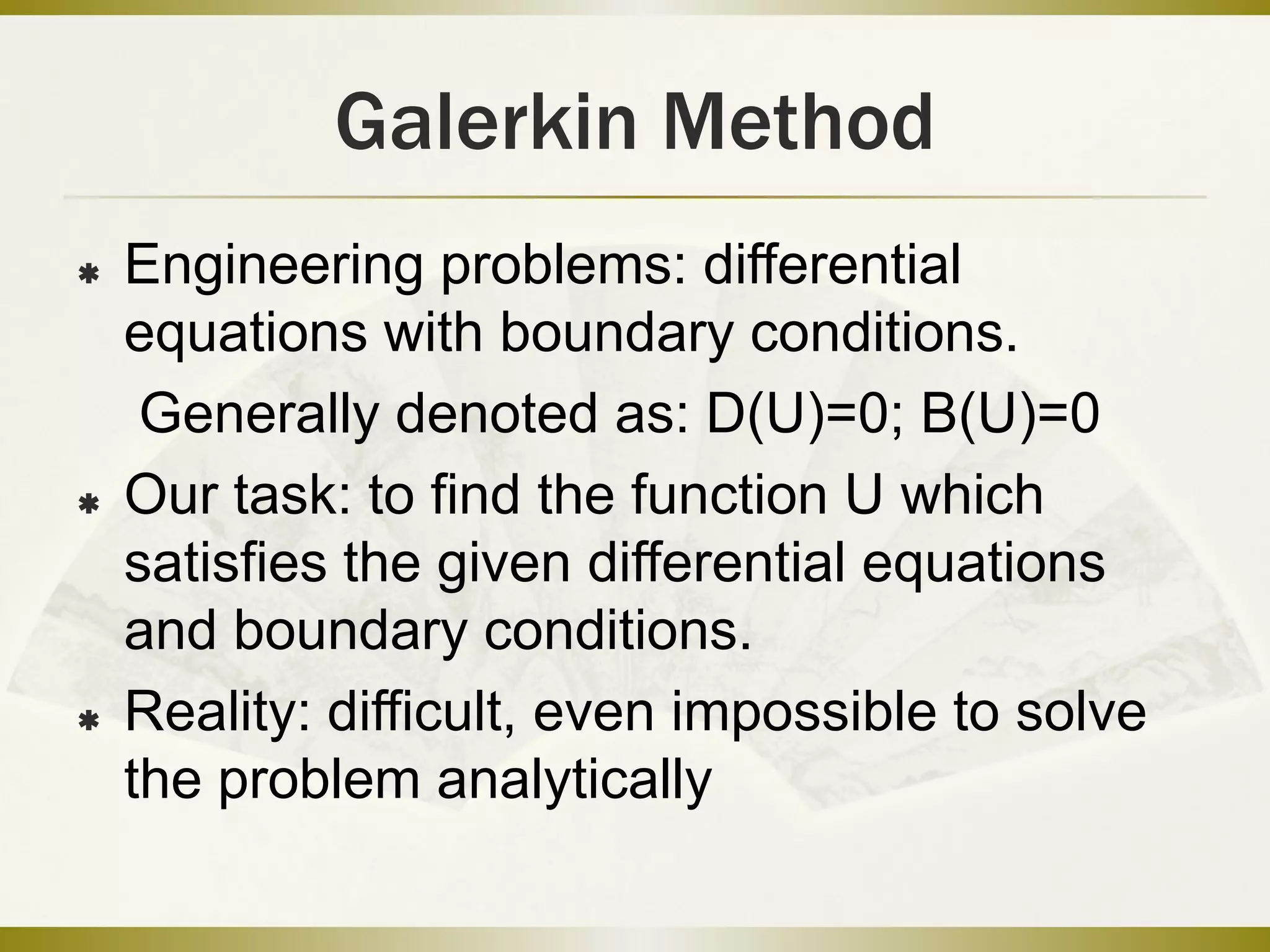
Computational Engineering
Galerkin Method
Yijian Zhan
Ning Ma
Galerkin Method
 Engineering problems: differential
equations with boundary conditions.
Generally denoted as: D(U)=0; B(U)=0
 Our task: to find the function U which
satisfies the given differential equations
and boundary conditions.
 Reality: difficult, even impossible to solve
the problem analytically
Galerkin Method
 In practical cases we often apply
approximation.
 One of the approximation methods:
Galerkin Method, invented by Russian
mathematician Boris Grigoryevich Galerkin.
Galerkin Method
Related knowledge
 Inner product of functions
 Basis of a vector space of functions
Galerkin Method
Inner product
 Inner product of two functions in a certain
domain:
shows the inner
product of f(x) and g(x) on the interval [ a,
b ].
*One important property: orthogonality
If , f and g are orthogonal to each
other;
**If for arbitrary w(x), =0, f(x) 0
, ( ) ( )
b
a
f g f x g x dx  
, 0f g 
,w f  
Galerkin Method
Basis of a space
 V: a function space
 Basis of V: a set of linear independent
functions
Any function could be uniquely
written as the linear combination of the
basis:
0{ ( )}i iS x 

( )f x V
0
( ) ( )j j
j
f x c x


 
Galerkin Method
Weighted residual methods
 A weighted residual method uses a finite
number of functions .
 The differential equation of the problem is
D(U)=0 on the boundary B(U), for example:
on B[U]=[a,b].
where “L” is a differential operator and “f”
is a given function. We have to solve the
D.E. to obtain U.
0{ ( )}n
i ix 
( ) ( ( )) ( ) 0D U L U x f x  
Galerkin method
Weighted residual
 Step 1.
Introduce a “trial solution” of U:
to replace U(x)
: finite number of basis functions
: unknown coefficients
* Residual is defined as:
0
1
( ) ( ) ( )
n
j j
j
U u x x c x 

   
jc
( )j x
( ) [ ( )] [ ( )] ( )R x D u x L u x f x  
Galerkin Method
Weighted residual
 Step 2.
Choose “arbitrary” “weight functions” w(x),
let:
With the concepts of “inner product” and
“orthogonality”, we have:
The inner product of the weight function
and the residual is zero, which means that
the trial function partially satisfies the
problem.
So, our goal: to construct such u(x)
, ( ) , ( ) ( ){ [ ( )]} 0
b
a
w R x w D u w x D u x dx   
Galerkin Method
Weighted residual
 Step 3.
Galerkin weighted residual method:
choose weight function w from the basis
functions , then
These are a set of n-order linear
equations. Solve it, obtain all of the
coefficients .
j
0
1
, [ ( )] ( ){ [ ( ) ( )]} 0
nb
j j j ja
j
w R D u dx x D x c x dx   

     
jc
Galerkin Method
Weighted residual
 Step 4.
The “trial solution”
is the approximation solution we want.
0
1
( ) ( ) ( )
n
j j
j
u x x c x 

  
Galerkin Method Example
 Solve the differential equation:
with the boundary condition:
( ( )) ''( ) ( ) 2 (1 ) 0D y x y x y x x x    
(0) 0, (1) 0y y 
Galerkin Method Example
 Step 1.
Choose trial function:
We make n=3, and
0
1
( ) ( ) ( )
n
i i
i
y x x c x 

  
0
1
2 2
2
3 3
3
0,
( 1),
( 1)
( 1)
x x
x x
x x





 
 
 
Galerkin Method Example
 Step 2.
The “weight functions” are the same as
the basis functions
Step 3.
Substitute the trial function y(x) into
i
0
1
, [ ( )] ( ){ [ ( ) ( )]} 0
nb
j j j ja
j
w R D u dx x D x c x dx   

     
Galerkin Method Example
 Step 4.
i=1,2,3; we have three equations with
three unknown coefficients1 2 3, ,c c c
31 2
31 2
31 2
43 51
0
15 10 84 315
615 111
0
70 84 630 13860
734 611
0
315 315 13860 60060
cc c
cc c
cc c
    
   
    
Galerkin Method Example
 Step 5.
Solve this linear equation set, get:
Obtain the approximation solution
1
2
3
1370
0.18521
7397
50688
0.185203
273689
132
0.00626989
21053
c
c
c
   
 
   
3
1
( ) ( )i i
i
y x c x

 
Galerkin Method Example
GalerkinGalerkin solutionsolution Analytic solutionAnalytic solution
References
 1. O. C. Zienkiewicz, R. L. Taylor, Finite
Element Method, Vol 1, The Basis, 2000
 2. Galerkin method, Wikipedia:
http://en.wikipedia.org/wiki/Galerkin_method#cite_note-BrennerScott-1

Galerkin method

  • 1.
  • 2.
    Galerkin Method  Engineeringproblems: differential equations with boundary conditions. Generally denoted as: D(U)=0; B(U)=0  Our task: to find the function U which satisfies the given differential equations and boundary conditions.  Reality: difficult, even impossible to solve the problem analytically
  • 3.
    Galerkin Method  Inpractical cases we often apply approximation.  One of the approximation methods: Galerkin Method, invented by Russian mathematician Boris Grigoryevich Galerkin.
  • 4.
    Galerkin Method Related knowledge Inner product of functions  Basis of a vector space of functions
  • 5.
    Galerkin Method Inner product Inner product of two functions in a certain domain: shows the inner product of f(x) and g(x) on the interval [ a, b ]. *One important property: orthogonality If , f and g are orthogonal to each other; **If for arbitrary w(x), =0, f(x) 0 , ( ) ( ) b a f g f x g x dx   , 0f g  ,w f  
  • 6.
    Galerkin Method Basis ofa space  V: a function space  Basis of V: a set of linear independent functions Any function could be uniquely written as the linear combination of the basis: 0{ ( )}i iS x   ( )f x V 0 ( ) ( )j j j f x c x    
  • 7.
    Galerkin Method Weighted residualmethods  A weighted residual method uses a finite number of functions .  The differential equation of the problem is D(U)=0 on the boundary B(U), for example: on B[U]=[a,b]. where “L” is a differential operator and “f” is a given function. We have to solve the D.E. to obtain U. 0{ ( )}n i ix  ( ) ( ( )) ( ) 0D U L U x f x  
  • 8.
    Galerkin method Weighted residual Step 1. Introduce a “trial solution” of U: to replace U(x) : finite number of basis functions : unknown coefficients * Residual is defined as: 0 1 ( ) ( ) ( ) n j j j U u x x c x       jc ( )j x ( ) [ ( )] [ ( )] ( )R x D u x L u x f x  
  • 9.
    Galerkin Method Weighted residual Step 2. Choose “arbitrary” “weight functions” w(x), let: With the concepts of “inner product” and “orthogonality”, we have: The inner product of the weight function and the residual is zero, which means that the trial function partially satisfies the problem. So, our goal: to construct such u(x) , ( ) , ( ) ( ){ [ ( )]} 0 b a w R x w D u w x D u x dx   
  • 10.
    Galerkin Method Weighted residual Step 3. Galerkin weighted residual method: choose weight function w from the basis functions , then These are a set of n-order linear equations. Solve it, obtain all of the coefficients . j 0 1 , [ ( )] ( ){ [ ( ) ( )]} 0 nb j j j ja j w R D u dx x D x c x dx           jc
  • 11.
    Galerkin Method Weighted residual Step 4. The “trial solution” is the approximation solution we want. 0 1 ( ) ( ) ( ) n j j j u x x c x     
  • 12.
    Galerkin Method Example Solve the differential equation: with the boundary condition: ( ( )) ''( ) ( ) 2 (1 ) 0D y x y x y x x x     (0) 0, (1) 0y y 
  • 13.
    Galerkin Method Example Step 1. Choose trial function: We make n=3, and 0 1 ( ) ( ) ( ) n i i i y x x c x      0 1 2 2 2 3 3 3 0, ( 1), ( 1) ( 1) x x x x x x           
  • 14.
    Galerkin Method Example Step 2. The “weight functions” are the same as the basis functions Step 3. Substitute the trial function y(x) into i 0 1 , [ ( )] ( ){ [ ( ) ( )]} 0 nb j j j ja j w R D u dx x D x c x dx          
  • 15.
    Galerkin Method Example Step 4. i=1,2,3; we have three equations with three unknown coefficients1 2 3, ,c c c 31 2 31 2 31 2 43 51 0 15 10 84 315 615 111 0 70 84 630 13860 734 611 0 315 315 13860 60060 cc c cc c cc c              
  • 16.
    Galerkin Method Example Step 5. Solve this linear equation set, get: Obtain the approximation solution 1 2 3 1370 0.18521 7397 50688 0.185203 273689 132 0.00626989 21053 c c c           3 1 ( ) ( )i i i y x c x   
  • 17.
    Galerkin Method Example GalerkinGalerkinsolutionsolution Analytic solutionAnalytic solution
  • 18.
    References  1. O.C. Zienkiewicz, R. L. Taylor, Finite Element Method, Vol 1, The Basis, 2000  2. Galerkin method, Wikipedia: http://en.wikipedia.org/wiki/Galerkin_method#cite_note-BrennerScott-1