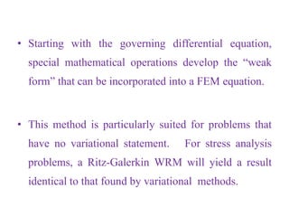
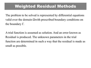
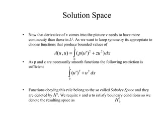
Weighted residual methods are used to solve differential equations numerically. They involve approximating the solution over the domain as a linear combination of basis functions. This creates a residual error that is minimized in an integral sense by choosing the coefficients to satisfy orthogonal conditions. Common weighted residual methods include Galerkin's method and point collocation. The weak form is preferred over the strong form as it requires less continuity from the test and trial functions.

1. Weighted Residual Methods

2. • Starting with the governing differential equation,
special mathematical operations develop the “weak
form” that can be incorporated into a FEM equation.
• This method is particularly suited for problems that
have no variational statement. For stress analysis
problems, a Ritz-Galerkin WRM will yield a result
identical to that found by variational methods.

3. Weighted Integral Forms
L
L
x
Q
dx
du
a
u
u
x
x
q
dx
du
x
a
dx
d
u
L








)
0
(
1
0
,
0
)
(
)
)
(
(
]
[
0
The class of differential equations containing also the one
dimensional bar described above can be described as follows
Here a(x) and q(x) are known functions of the coordinate x.
uo and QL are known parameters.
L is the size of the one dimensional domain of the problem.
When the specified values of uo and QL are nonzero the
boundary conditions are said to be nonhomogeneous
When uo =0 and QL =0 the boundary conditions are said to
be homoheneous

4. Approximating Function
Suppose we seek an approximation
The functions fj is of our choice and is meant to be suitable to the
particular problem. For example the choice of sine and cosine
functions satisfy boundary conditions hence it could be a good choice.
Now determine cj such that U(x) satisfies the differential equation
Since the LHS of the equation now is an approximate value we will
get a quantity R≠0 called Residual on the RHS




N
j
j
j x
c
x
U
x
u
1
)
(
)
(
)
( f
.
)
)
(
( R
q
dx
dU
x
a
dx
d



5. Weighted Integral Forms
The residue R is made equal to zero in a weighted integral sense as
Where w(x) is a weighting function
This is the weighted integral form
 
L
dx
x
R
x
w
0
0
)
(
)
(

6. Weighted Residual Methods
The problem to be solved is represented by differential equations
valid over the domain Ωwith prescribed boundary conditions on
the boundary Γ.
A trial function is assumed as solution. And an error known as
Residual is produced. The unknown parameters in the trial
function are determined in such a way that the residual is made as
small as possible.

7. Weighted Residual Methods
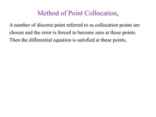
It follows that:
Multiplying this by a weight function w and integrating over the
whole domain we obtain:
Some of the most commonly used weighted residual methods are
Method of Point Collocation,
Method of Least squares,
Method of Subdomain Collocation and
Galerkin’s method
R
q
U
L 

]
[
 

1
0
0
)
]
[
( dx
w
q
u
L

8. Method of Point Collocation,
A number of discrete point referred to as collocation points are
chosen and the error is forced to become zero at these points.
Then the differential equation is satisfied at these points.

9. Approximating Function
• We can replace u and v in the formula with their approximation
function i.e.
• The functions fj and yj are of our choice and are meant to be suitable
to the particular problem. For example the choice of sine and cosine
functions satisfy boundary conditions hence it could be a good
choice.








N
j
j
j
N
j
j
j
x
d
x
V
x
v
x
c
x
U
x
u
1
1
)
(
)
(
)
(
)
(
)
(
)
(
y
f

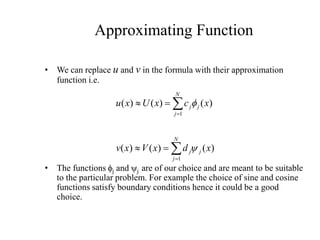
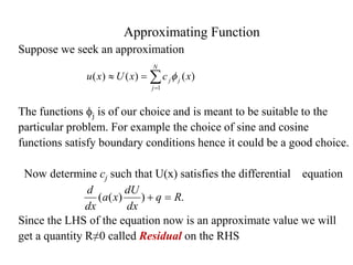
10. 4.2 Approximating Function
• U is called trial function and V is called test function
• As the differential operator L[u] is second order
• Therefore we can see U as element of a finite-diemnsional
subspace of the infinite-dimensional function space C2(0,1)
• The same way
)
1
,
0
(
)
1
,
0
( 2
2
C
U
C
u 


)
1
,
0
(
)
1
,
0
( 2
C
S
U N


)
1
,
0
(
)
1
,
0
(
ˆ 2
L
S
V N



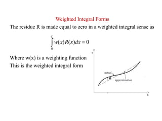
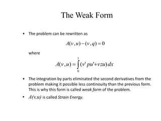
11. • Replacing v and u with respectively V and U (2) becomes
• r(x) is called the residual (as the name of the method suggests)
• The vanishing inner product shows that the residual is orthogonal to all
functions V in the test space.
q
U
L
x
r
S
V
r
V N





]
[
)
(
ˆ
,
0
)
,
(
The Residual

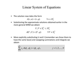
12. • Substituting into
and exchanging summations and integrals we obtain
• As the inner product equation is satisfied for all choices of V in SN
the above equation has to be valid for all choices of dj which implies
that
The Residual



N
j
j
j x
d
x
V
1
)
(
)
( y 0
)
]
[
,
( 
 q
U
L
V
N
j
d
q
U
L
d j
N
j
j
j ,
...
,
2
,
1
,
0
)
]
[
,
(
1






y
N
j
q
U
L
j ,
...
,
2
,
1
0
)
]
[
,
( 


y

13. • One obvious choice of would be taking it equal to
• This Choice leads to the Galerkin’s Method
• This form of the problem is called the strong form of the problem.
Because the so chosen test space has more continuity than
necessary.
• Therefore it is worthwile for this and other reasons to convert the
problem into a more symmetrical form
• This can be acheived by integrating by parts the initial strong form
of the problem.
Galerkin’s Method
j
y j
f
N
j
q
U
L
j ,
...
,
2
,
1
0
)
]
[
,
( 


f

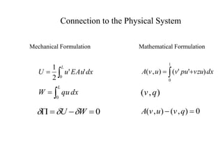
14. • Let us remember the initial form of the problem
• Integrating by parts
The Weak Form
dx
q
zu
pu
v
q
u
L
v  




1
0
]
)'
'
(
[
)
]
[
,
(
.
0
)
1
(
)
0
(
1
0
),
(
)
(
)
)
(
(
]
[








u
u
x
x
q
u
x
z
dx
du
x
p
dx
d
u
L
0
'
)
'
'
(
]
)'
'
(
[
1
0
1
0
1
0







 
 vpu
dx
vq
vzu
pu
v
dx
q
zu
pu
v

15. The Weak Form
• The problem can be rewritten as
where
• The integration by parts eliminated the second derivatives from the
problem making it possible less continouity than the previous form.
This is why this form is called weak form of the problem.
• A(v,u) is called Strain Energy.
0
)
,
(
)
,
( 
 q
v
u
v
A
dx
vzu
pu
v
u
v
A )
'
'
(
)
,
(
1
0
 


16. Solution Space
• Now that derivative of v comes into the picture v needs to have more
continoutiy than those in L2. As we want to keep symmetry its appropriate to
choose functions that produce bounded values of
• As p and z are necessarily smooth functions the following restriction is
sufficient
• Functions obeying this rule belong to the so called Sobolev Space and they
are denoted by H1. We require v and u to satisfy boundary conditions so we
denote the resulting space as
dx
zu
u
p
u
u
A )
)
'
(
(
)
,
(
1
0
2
2
 

1
0
1
0
2
2
)
'
(
H
dx
u
u
 

17. • The solution now takes the form
• Substituting the approximate solutions obtained earlier in the
more general WRM we obtain
• More explicitly substituting U and V (remember we chose them to
have the same base) and swapping summations and integrals we
obtain
Linear System of Equations
1
0
)
,
(
)
,
( H
v
q
v
u
v
A 


N
N
S
V
q
V
U
V
A
H
S
V
U
0
1
0
0
)
,
(
)
,
(
,









N
k
j
k
j
k N
j
q
A
c
1
,
...
,
2
,
1
,
)
,
(
)
,
( f
f
f

18. Connection to the Physical System
Mechanical Formulation Mathematical Formulation
dx
EAu
u
U
L


0
'
'
2
1


L
dx
qu
W
0
0



 W
U 


dx
vzu
pu
v
u
v
A )
'
'
(
)
,
(
1
0
 

0
)
,
(
)
,
( 
 q
v
u
v
A
)
,
( q
v

19. Weak Formulation for Beam Element
• Governing Equation
,
0
)
(
2
2
2
2










f
dx
x
v
d
EI
dx
d
• Weighted-Integral Formulation for one element
 















2
1
)
(
)
(
)
(
0 2
2
2
2
x
x
dx
x
q
dx
x
v
d
EI
dx
d
x
w
• Weak Form from Integration-by-Parts ----- (1st time)
2
1
2
1
2
2
2
2
0
x
x
x
x
dx
v
d
EI
dx
d
w
dx
wq
dx
v
d
EI
dx
d
dx
dw

























 
L
x 

0

20. Beam Element
Deflection of Elastic Beams
Using Euler-Bernouli Theory
1 2
w1
w2
q2
q1
)
(
,
,
,
:
ion
Specificat
Condtions
Boundary
)
(
)
(
:
Equation
al
Differenti
2
2
2
2
2
2
2
2
dx
w
d
b
dx
d
dx
w
d
b
dx
dw
w
x
f
dx
w
d
b
dx
d

