Fuzzy Regression Model.

Fuzzy Regression Models
Arnold F. Shapiro
Penn State University
Smeal College of Business, University Park, PA 16802, USA
Phone: 01-814-865-3961, Fax: 01-814-865-6284, E-mail: afs1@psu.edu
Abstract
Recent articles, such as McCauley-Bell et al. (1999) and Sánchez and Gómez (2003a,
2003b, 2004), used fuzzy regression (FR) in their analysis. Following Tanaka et. al.
(1982), their regression models included a fuzzy output, fuzzy coefficients and an non-
fuzzy input vector. The fuzzy components were assumed to be triangular fuzzy numbers
(TFNs). The basic idea was to minimize the fuzziness of the model by minimizing the
total support of the fuzzy coefficients, subject to including all the given data.
The purpose of this article is to revisit the fuzzy regression portions of the foregoing
studies and to discuss issues related to the Tanaka approach, including a consideration of
fuzzy least-squares regression models.
Keywords: fuzzy linear regression, fuzzy least-squares regression, fuzzy coefficients,
possibilistic regression, term structure of interest rates
Acknowledgments:
This work was supported in part by the Robert G. Schwartz Faculty Fellowship and the
Smeal Research Grants Program at the Penn State University. The assistance of Michelle
L. Fultz is gratefully acknowledged.
© 2005 Arnold F. Shapiro. All rights reserved.
ARC2005_Shapiro_06.pdf 1

1 Introduction
Recent articles, such as McCauley-Bell et al. (1999) and Sánchez and Gómez (2003a,
2003b, 2004), used fuzzy regression (FR) in their analysis. The former use it to predict
the relationship of known risk factors to the onset of occupational injury, while the latter
used it to investigate the term structure of interest rates (TSIR). Following Tanaka et. al.
(1982), their models took the general form:
nn xAxAAY
~~~~
110 +++= L (1)
where Y
~
is the fuzzy output, Ãi, j=1,2,..., n, is a fuzzy coefficient, and x = (x1, ..., xn) is an
n-dimensional non-fuzzy input vector. The fuzzy components were assumed to be
triangular fuzzy numbers (TFNs). Consequently, the coefficients, for example, can be
characterized by a membership function (MF), µA(a), a representation of which is shown
in Figure 1.
Figure 1: Fuzzy Coefficient
As indicated, the salient features of the TFN are its mode, its left and right spread, and its
support. When the two spreads are equal, the TFN is known as a symmetrical TFN
(STFN).
The basic idea of the Tanaka approach, often referred to as possibilistic regression, was to
minimize the fuzziness of the model by minimizing the total spread of the fuzzy
coefficients, subject to including all the given data.
The purpose of this article is to revisit the fuzzy regression portions of the foregoing
studies, and to discuss issues related to the Tanaka (possibilistic) regression model. This

discussion is not meant to be exhaustive but, rather, is intended to point out some of the
major considerations. The outline of the paper is as follows. We first define and
conceptualize the general components of fuzzy regression. Next, the essence of the
Tanaka model is explored, including a commentary on some of its potential limitations.
Then, fuzzy least-squares regression models are discussed as an alternative to the Tanaka
model. Throughout the paper, the same simple data set is used to show how the ideas are
implemented. The paper ends with a summary of the conclusions of the study.
2 Fuzzy Linear Regression Basics
This section provides an introduction to fuzzy linear regression. The topics addressed
include the motivation for FR, the components of FR, fuzzy coefficients, the h-certain
factor, and fuzzy output.
2.1 Motivation
Classical statistical linear regressions takes the form
(2)mixxy iikkii ,...,2,1,110 =++++= εβββ L
where the dependent (response) variable, yi , the independent (explanatory) variables, xij,
and the coefficients (parameters), βj, are crisp values, and εi is a crisp random error term
with E(εi)=0, variance σ2
(εi )=σ2
, and covariance σ(εi , εj) = 0, ∀i,j, i≠ j.
Although statistical regression has many applications, problems can occur in the
following situations:
• Number of observations is inadequate (Small data set)
• Difficulties verifying distribution assumptions
• Vagueness in the relationship between input and output variables
• Ambiguity of events or degree to which they occur
• Inaccuracy and distortion introduced by linearalization
Thus, statistical regression is problematic if the data set is too small, or there is difficulty
verifying that the error is normally distributed, or if there is vagueness in the relationship
between the independent and dependent variables, or if there is ambiguity associated with
the event or if the linearity assumption is inappropriate. These are the very situations
fuzzy regression was meant to address.
2.2 The Components of Fuzzy Regression
There are two general ways (not necessarily mutually exclusive) to develop a fuzzy
regression model: (1) models where the relationship of the variables is fuzzy; and (2)

models where the variables themselves are fuzzy. Both of these models are explored in
the rest of this article, but, for this conceptualization, we focus on models where the data
is crisp and the relationship of the variables is fuzzy.
It is a simple matter to conceptualize fuzzy regression. Consider for this, and subsequent,
examples the following simple Ishibuchi (1992) data:
Table 1: Data Pairs
i 1 2 3 4 5 6 7 8
xi 2 4 6 8 10 12 14 16
yi 14 16 14 18 18 22 18 22
Starting with this data, we fit a straight line through two or more data points in such a
way that it bounds the data points from above. Here, these points are determined
heuristically and OLS is used to compute the parameters of the line labeled YH
, which
takes the values , as shown in Figure 2(a).xy 75.13ˆ +=
Figure 2: Conceptualizing the upper and lower bound
Similarly, we fit a second straight line through two or more data points in such a way that
it bounds the data points from below. As shown in Figure 2(b), the fitted line in
this case is labeled YL
and takes the values xy 5.11ˆ += .
Assuming, for the purpose of this example, that STFN are used for the MFs, the modes of
the MFs fall midway between the boundary lines.1
1
This approach to choosing the mode was discussed by Wang and Tsaur (2000) p. 357.

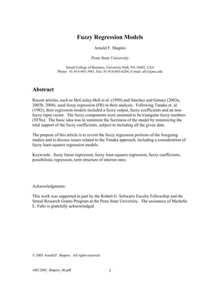
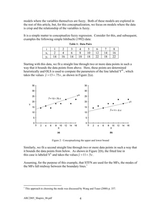
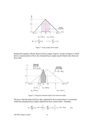
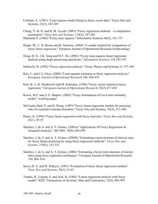
For any given data pair, (xi, yi), the foregoing conceptualizations can be summarized by
the fuzzy regression interval [Y shown in Figure 3.]Y, U
i
L
i
2
Figure 3: Fuzzy Regression Interval
1h
iY =
is the mode of the MF and if a SFTN is assumed, )/2Y(YY L
i
U
ii
1h
i +===
)Y,Y, 1h
i
L
i
U
i
=
L
iY
Y . Given
the parameters, (YU
,YL
, Yh=1
), which characterize the fuzzy regression model, the i-th
data pair (xi,yi), is associated with the model parameters (Y . From a
regression perspective, we can view - yU
iY
U
iY -
i and yi - as components of the SST, yL
iY
1h
i
=
i -
as a component of SSE, and and - as components of the SSR, as
discussed by Wang and Tsaur (2000).
1h
iY = 1h
iY =
Y
In possibilistic regression based on STFN, only the data points involved in determining
the upper and lower bounds determine the structure of the model, as depicted in Figure 2.
The rest of the data points have no impact on the structure. This problem is resolved by
using asymmetric TFNs.
2.3 The Fuzzy Coefficients
Combining Equation (1) and Figure 1, and, for the present, restricting the discussion to
STFNs, the MF of the j-th coefficient, may be defined as:







 −
−= 0,
||
1max)(
j
j
A
c
aa
aj
µ (3)
where aj is the mode and cj is the spread, and represented as shown in Figure 4.
2
Adapted from Wang and Tsaur (2000), Figure 1.

Figure 4: Symmetrical fuzzy parameters
Defining
(
{ } { } njcaAcaAcaA LjjjjjjLjjj ,,1,0,
~
:
~
,
~
L=+≤≤−== (4)
and restricting consideration to the case where only the coefficients are fuzzy, we can
write
5)
∑=
+=
n
j
iji xAAY
1
10
~~~
∑=
+=
n
j
ijLjjL xcaca
1
00 ),(),(
This is a useful formulation because it explicitly portrays the mode and spreads of the
fuzzy parameters. In a subsequent section, we explore fuzzy independent variables.
2.4 The "h-certain" Factor
If, as in Figure 3, the supports3
are just sufficient to include all the data points of the
sample, there would be only limited confidence in out-of-sample projection using the
estimated FR model. This is resolved for FR, just as it is with statistical regression, by
extending the supports.
Consider the MF associated with the j-th fuzzy coefficient, a representation of which is
shown in Figure 5.
3
Support functions are discussed in Diamond (1988: 143) and Wünsche and Näther (2002: 47).

Figure 5: Estimating Aj using an "h-certain" factor
For illustrative purposes, a non-symmetric TFN is shown, wherec andc represent the
left and right spread respectively. Beyond that, what makes this MF materially different
from the one shown in Figure 4, is that it contains a point "h" on the y-axis, called an "h-
certain factor," which, by controlling the size of the feasible data interval (the base of the
shaded area), extends the support of the MF.
L
j
R
j
4
In particular, as the h-factor increases for a
given data set, so increases the spreads,c and .L
j
R
jc
2.5 Observed Fuzzy Output
An h-certain factor also can be applied to the observed output. Thus, the i-th output data
might be represented by the STFN, )e,(yY
~
iii = , where yi is the mode and ei is the spread,
as shown in Figure 6. Here, the actual data points fall within the interval yi ± (1-h) ei, the
base of the shaded portion of the graph.
4
Note that the h-factor has the opposite purpose of an α-cut, in that the former is used to extend the
support, while the latter is used to reduce the support.

Figure 6: Observed Fuzzy Output
2.6 Fitting the Fuzzy Regression Model
Given the foregoing, two general approaches are used to fit the fuzzy regression model:
The possibilistic model. Minimize the fuzziness of the model by minimizing the total
spreads of its fuzzy coefficients (see Figure 1), subject to including the data points of
each sample within a specified feasible data interval.
The least-squares model. Minimize the distance between the output of the model and
the observed output, based on their modes and spreads.
The details of these approaches are addressed in the next two sections of this paper.
3 The Possibilistic Regression Model
The possibilistic regression model is optimized by minimizing the spread, subject to
adequate containment of the data. The spread is minimized
0c,|x|ccmin j
n
1j
ijj0 ≥





+ ∑=
(6)
Figure 7 shows the first step in the containment requirement, by showing how Figure 5
can be easily extended to portray the fuzzy output of the model.

Figure 7: Fuzzy output of the model
Putting this together with the observed fuzzy output, Figure 6, results in Figure 8, which
shows a representation of how the estimated fuzzy output may be fitted to the observed
fuzzy data.
Figure 8: Fitting the estimated output to the observed output
The key is that the observed fuzzy data, adjusted for the h-certain factor, is contained
within the estimated fuzzy output, adjusted for the h-certain factor. Formally,
ii
n
j
n
j
ijjijj ehyxcchxaa )1(||)1(
1 1
00 −+>





+−++∑ ∑= =
(7)

ii
n
j
n
j
ijjijj ehyxcchxaa )1(||)1(
1 1
00 −−<





+−−+∑ ∑= =
cj $0, i = 0, 1, ..., m, j = 0, 1, ..., n
Figure 95
shows the impact of the h-factor on the sample data, given h=0 and h=.7.
Figure 9: FLR and h-certain model
The result is what one would expect. Increasing the h-factor expands the confidence
interval and, thus, increases the probability that out-of-sample values will fall within the
model. This is comparable to increasing the confidence in statistical regression by
increasing the confidence interval.
The possibilistic linear regression model, as depicted by equations (6) and (7), is
essentially the fuzzy regression model used by Sánchez and Gómez (2003a, 2003b, 2004)
to investigate the TSIR.6
5
Adapted from Chang and Ayyub (2001), Figure 4.
6
Key components of the Sánchez and Gómez methodology included constructing a discount function from
a linear combination of quadratic or cubic splines, the coefficients of which were assumed to be TFNs or
STFNs, and using the minimum and maximum negotiated price of fixed income assets to obtain the spreads
of the dependent variable observations. Given the fuzzy discount functions, the authors provided TFN
approximations for the corresponding spot rates and forward rates. It was necessary to approximate the
spot rates and forward rates since they are nonlinear functions of the discount function, and hence are not
TFNs even though the discount function is a TFN.

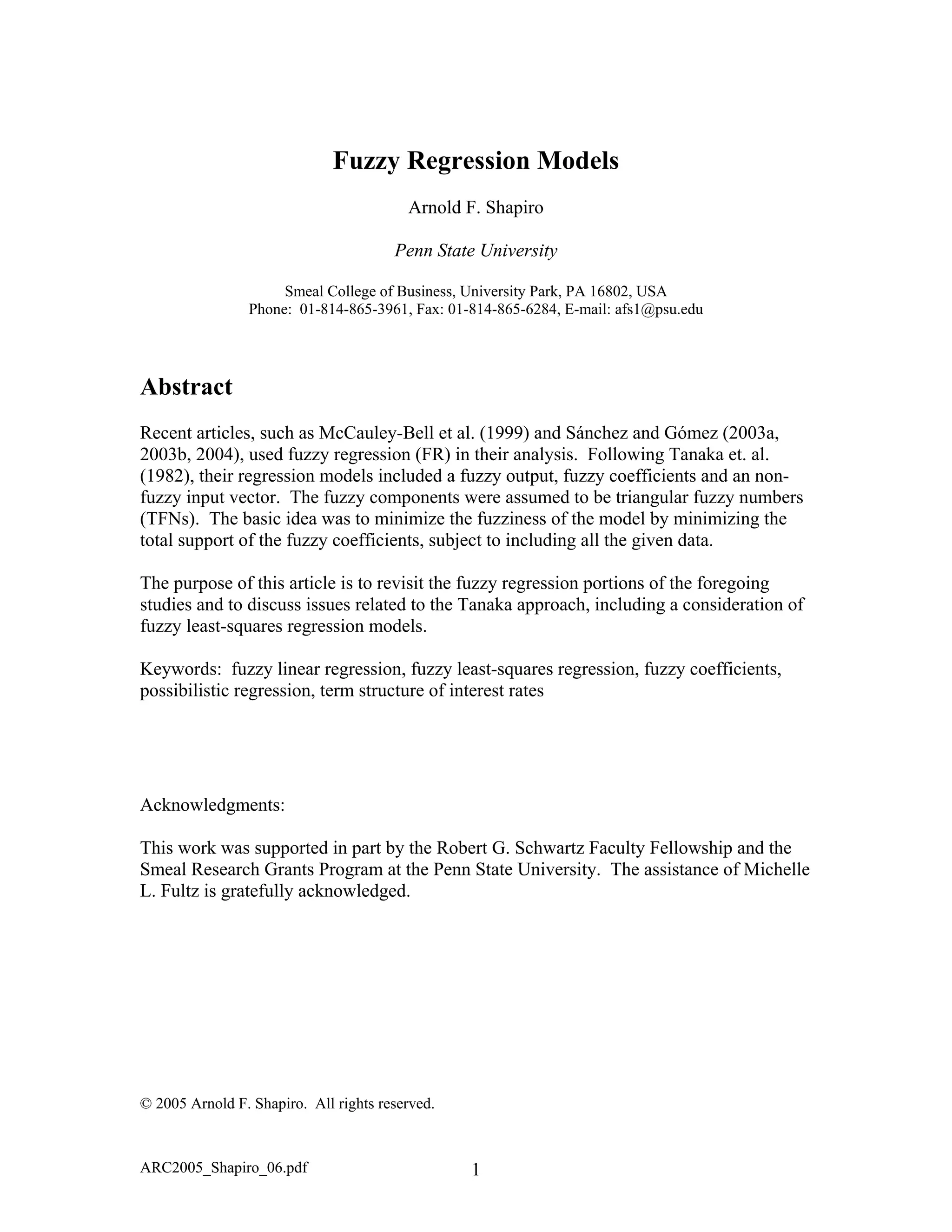
3.1 Criticisms of the Possibilistic Regression Model
There are a number of criticisms of the possibilistic regression model. Some of the major
ones are the following:
• Tanaka et al "used linear programming techniques to develop a model superficially
resembling linear regression, but it is unclear what the relation is to a least-squares
concept, or that any measure of best fit by residuals is present." [Diamond (1988:
141-2)]
• The original Tanaka model was extremely sensitive to the outliers. [Peters (1994)].
• There is no proper interpretation about the fuzzy regression interval [Wang and
Tsaur (2000)]
• Issue of forecasting have to be addressed [Savic and Pedrycz (1991)]
• The fuzzy linear regression may tend to become multicollinear as more independent
variables are collected [Kim et al (1996)].
• The solution is xj point-of-reference dependent, in the sense that the predicted
function will be very different if we first subtract the mean of the independent
variables, using (xj - ix ) instead of xj. [Hojati (2004), Bardossy (1990) and Bardossy
et al (1990)]
4 The Fuzzy Least-Squares Regression (FLSR) Model
An obvious way to bring the FR more in line with statistical regression is to model the
fuzzy regression along the same lines. In the case of a single explanatory variable, we
start with the standard linear regression model: [Kao and Chyu (2003)]
(8)m1,2,...,i,εxββy ii10i =++=
which in a comparable fuzzy model might take the form:
m1,2,...,i,ε~X
~
ββY
~
ii10i =++= (9)
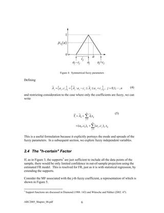
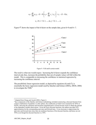
Conceptually, the relationship between the fuzzy i-th response and explanatory variables
in (9) can be represented as shown in Figure 10.

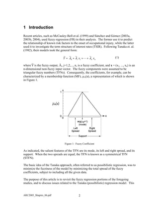
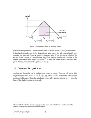
Figure 10: Fuzzy i-th response and explanatory variables
Rearranging the terms in (9),
m1,2,...,i,X
~
ββY
~
ε~
i10ii =−−= (10)
From a least-squares perspective, the problem then becomes
2
10
1
)
~~
(min i
n
i
i XbbY −−∑
=
(11)
There are a number of ways to implement FLSR, but the two basic approaches are FLSR
using distance measures and FLSR using compatibility measures. A description of these
methods follows.
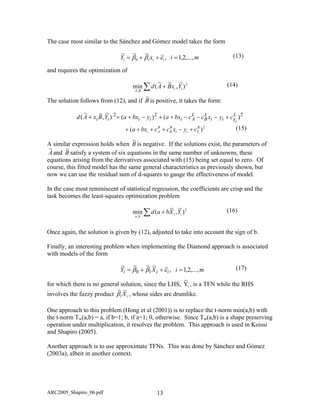
4.1 FLSR using Distance Measures (Diamond's Approach)
Diamond (1988) was the first to implement the FLSR using distance measures and his
methodology is the most commonly used. Essentially, he defined an L2
- metric d(.,.)2
between two TFNs by [Diamond (1988: 143) equation (2)]
(12)( ) ( )
( )2
2211
2
2211
2
21
2
222111
)()(
)()()(,,,,,
rmrm
lmlmmmrlmrlmd
+−++
−−−+−=
Given TFNs, it provides a measure of the distance between two fuzzy numbers based on
their modes, left spread and right spread.7
7
The methods of Diamond's paper are rigorously justified by a projection-type theorem for cones on a
Banach space containing the cone of triangular fuzzy numbers, where a Banach space is a normed vector
space that is complete as a metric space under the metric d(x, y) = ||x-y|| induced by the norm.

The case most similar to the Sánchez and Gómez model takes the form
mixY iii ,...,2,1,~~~~
10 =++= εββ (13)
and requires the optimization of
2
,
)
~
,
~~
(min ii
BA
YxBAd∑ + (14)
The solution follows from (12), and if B
~
is positive, it takes the form:
222
)()()
~
,
~~
( L
Yii
L
B
L
Aiiiii i
cyxccbxaybxaYBxAd +−−−++−+=+
(15)
A similar expression holds when
2
)( R
Yii
R
B
R
Ai i
cyxccbxa +−++++
B
~
is negative. If the solutions exist, the parameters of
A
~
and B
~
course, this fitted model has the same general characteristics as previously shown, but
now we can use the residual sum of d-squares to gauge the effectiveness of model.
In the case most reminiscent of statistical regression, the coefficients are crisp and the
task becomes the least-squares optimization problem
satisfy a system of six equations in the same number of unknowns, these
quations arising from the derivatives associated with (15) being set equal to zero. Of
(16)
Once again, the solution is gi to account t n of b.
Finally, an interesting problem enting the Diamond approach is associated
ith models of the form
ral solution, since the LHS,
e
,
)
~
,
~
(min ii
ba
YXbad∑ + 2
ven by (12), adjusted to take
when implem
in he sig
w
(17)
for which there is no gene
miXY iii ,...,2,1,10 =++= εββ ~~~~~
iY
~
One approach to this problem (Hong et al (2001)) is to replace the t-norm min(a,b)
the t-norm Tw(a,b) = a, if b=1; b, if a=1; 0, otherwise. Since T
, is a TF while the RHS
involves the fuzzy product
N
iX
~~
1β , whose sides are drumlike.
with
w(a,b) is a shape preserving
peration under multiplication, it resolves the problem. This approach is used in Koissio
and Shapiro (2005).
Another approach is to use approximate TFNs. This was done by Sánchez and Gómez
(2003a), albeit in another context.

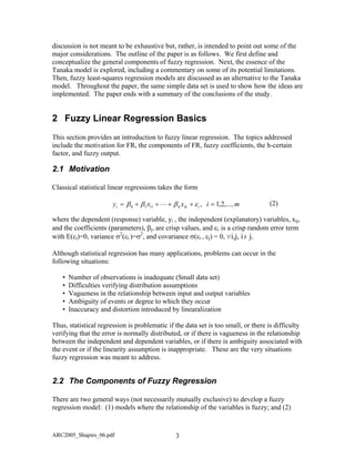
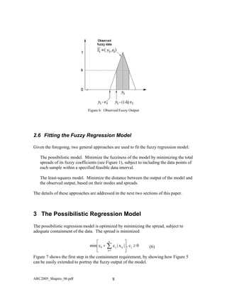
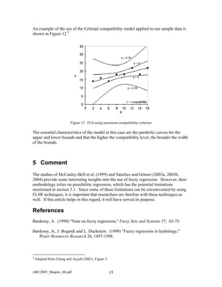
4.2 FLSR using compatibility measures
An alternate least-squares approach is based on the Celmiņš (1987) compatibility
(18)
As indicated, when the
odes of the MFs coincide.
elmiņš compatibility model, which involved maximizing the compatibility between the
(19)
Thus, for example, when there is a single crisp expla
(2001: 190)]
(20)
m1 are determined using weighted LS regression, and c0, c1, and c01 are
determined using iteration and the desired compatibility measure.
measure
(),(min{max)
~
,
~
( XBA µµγ =
representative examples of which are shown in Figure 11.8
Figure 11: Celmiņš Compatibility Measure
γ ranges from 0, when the MFs are mutually exclusive, to 1,
m
C
data and the fitted model, follows from this measure. The objective function is
natory variable, [Chang and Ayyub
1=
−
m
iγ
i
)}XBA
x
2
)1(∑
22
101010
10
2
~~ˆ
xcxccxmm
xAAY
++±+=
+=
where m0 and
8

An example of the use of the Celmiņš compatibility model applied to our sample data is
own in Figure 12.9
The essential characte rves for the
e broader the width
of the bounds.
cCauley-Bell et al. (1999) and Sánchez and Gómez (2003a, 2003b,
004) provide some interesting insights into the use of fuzzy regression. However, their
ethodology relies on possibilitic regression, which has the potential limitations
1. Since some of these limitations can be circumvented by using
mportant that researchers are familiar with these techniques as
ell. If this article helps in this regard, it will have served its purpose.
hydrology,"
Water Resources Research 26, 1497-1508.
sh
Figure 12: FLS using maximum compatibility criterion
ristics of the model in this case are the parabolic cu
upper and lower bounds and that the higher the compatibility level, th
5 Comment
The studies of M
2
m
mentioned in section 3.
FLSR techniques, it is i
w
References
Bardossy, A. (1990) "Note on fuzzy regression," Fuzzy Sets and Systems 37, 65-75.
Bardossy, A., I. Bogardi and L. Duckstein. (1990) "Fuzzy regression in
9

Celmiņš, A. (1987) "Least squares model fitting to fuzzy vector data," Fuzzy Sets and
Systems, 22(3), 245-269
Cha zy regression methods – a comparative
assessment," Fuzzy Sets and Systems, 119(2), 187-203
ojati, M., C. R. Bector and K. Smimou. (2004) "A simple method for computation of
n
analysis using shape preserving operations," Information Sciences 138 185-193
Ish 8
"
regression," European Journal of Operational Research, 92(2) 417-434
Koi ee-Carter mortality
model,” working paper.
Mc assessing
risks of cumulative trauma disorders," Fuzzy Sets and Systems, 92(3), 317-340
Peters, G. (1994) "Fuzzy linear regression with fuzzy intervals," Fuzzy Sets and Systems,
63(1), 45-55
Sán
Actuarial Analysis," JRI 2003, 70(4), 665-699
Sánchez, J. de A. and A. T. Gómez. (2003b) "Estimating a term structure of interest rates
for fuzzy financial pricing by using fuzzy regression methods," Fuzzy Sets and
ánchez, J. de A. and A. T. Gómez. (2004) "Estimating a fuzzy term structure of interest
Savic, D. A. and W. Pedrycz. (1991) "Evaluation of fuzzy linear regression models,"
Tan nd Asai, K. (1982) "Linear regression analysis with fuzzy
model," IEEE Transactions on Systems, Man and Cybernetics, 12(6), 903-907.
ng, Y.-H. O. and B. M. Ayyub. (2001) "Fuz
Diamond, P. (1988) "Fuzzy least squares," Information Sciences 46(3), 141-157
H
fuzzy linear regression," European Journal of Operational Research (forthcoming)
Hong, D. H., J-K. Song and H.Y. Do. (2001) "Fuzzy least-squares linear regressio
ibuchi, H. (1992) "Fuzzy regression analysis," Fuzzy Theory and Systems, 4, 137-14
Kao, C. and C-L Chyu. (2003) "Least-squares estimates in fuzzy regression analysis,
European Journal of Operational Research 148, 426-435
Kim, K. J., H. Moskowitz and M. Koksalan. (1996) "Fuzzy versus statistical linear
ssi, M-C and A. F. Shapiro. (2005) “Fuzzy formulation of L
Cauley-Bell, P. and H. Wang. (1997) "Fuzzy linear regression models for
chez, J. de A. and A. T. Gómez. (2003a) "Applications Of Fuzzy Regression In
Systems, 139(2), 313-331
S
rates using fuzzy regression techniques," European Journal of Operational Research
154, 804–818
Fuzzy Sets and Systems, 39(1), 51-63
aka, H., Uejima, S. a

ng, H.-F. and R.-C. Tsaur. (2000) "InsiWa ght of a fuzzy regression model," Fuzzy Sets
and Systems, 112(3), 355-369
Wü dom
variables," Fuzzy Sets and Systems, 130(1), 43-50
nsche, A. and W. Näther. (2002) "Least-squares fuzzy regression with fuzzy ran

Fuzzy Regression Model.

Recommended

Recommended

More Related Content

What's hot

What's hot (20)

Viewers also liked

Viewers also liked (9)

Similar to Fuzzy Regression Model.

Similar to Fuzzy Regression Model. (20)

More from Dr. Volkan OBAN

More from Dr. Volkan OBAN (20)

Recently uploaded

Recently uploaded (20)

Fuzzy Regression Model.