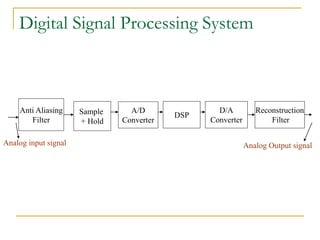
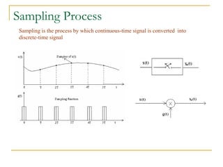
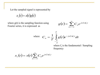
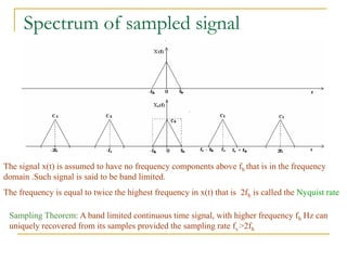
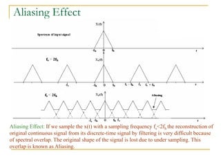
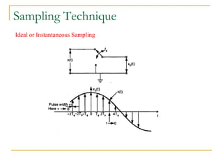
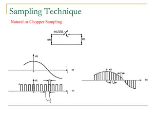
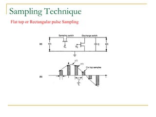
The document provides an overview of the processes involved in analog to digital conversion, emphasizing the sampling process and the importance of adhering to the Nyquist rate to avoid aliasing. It explains the quantization step and error, detailing how continuous-time signals are converted into discrete-time signals. Additionally, various sampling techniques and the characteristics of sampled signals are discussed with reference to Fourier analysis.

1. ANALOG TO DIGITAL
CONVERSION

2. Digital Signal Processing System
Anti Aliasing
Filter
Sample
+ Hold
A/D
Converter
DSP
D/A
Converter
Reconstruction
Filter
Analog input signal Analog Output signal

3. Analog to Digital Converter
Continuous- time
Continuous- amplitude
input signal
SAMPLER QUANTIZER ENCODER
Discrete-time
Continuous-
amplitude signal
Discrete-time Discrete
amplitude signal
Digital
Output
signal

4. Sampling Process
Sampling is the process by which continuous-time signal is converted into
discrete-time signal

5.   




n
t
f
jn
n
s
e
C
t
g 
2
  dt
e
t
g
T
C
T
T
t
f
jn
n
s




2
2
2
1 
   




n
t
f
jn
n
s
s
e
C
t
x
t
x 
2
     
t
g
t
x
t
xs 
Let the sampled signal is represented by
where g(t) is the sampling function using
Fourier series, it is expressed as
where
where fs is the fundamental / Sampling
frequency

6.     dt
e
e
t
x
C
f
X ft
j
t
f
jn
n
n
s
s
 







 
 2
2
   






n
s
n
s nf
f
X
C
f
X
     
1
2













 




dt
e
t
x
f
X ft
j
s
s

Using Fourier transform the spectrum of xs(t) is denoted by
Substituting xs(t) in the above equation,
Thus by comparing
with eqn 1
   




n
t
f
jn
n
s
s
e
C
t
x
t
x 
2
     
 








n
t
nf
f
j
n
s dt
e
t
x
C
f
X s

2

7. Spectrum of sampled signal
The signal x(t) is assumed to have no frequency components above fh that is in the frequency
domain .Such signal is said to be band limited.
The frequency is equal to twice the highest frequency in x(t) that is 2fh is called the Nyquist rate
Sampling Theorem: A band limited continuous time signal, with higher frequency fh Hz can
uniquely recovered from its samples provided the sampling rate fs >2fh

8. Aliasing Effect
Aliasing Effect: If we sample the x(t) with a sampling frequency fs<2fh the reconstruction of
original continuous signal from its discrete-time signal by filtering is very difficult because
of spectral overlap. The original shape of the signal is lost due to under sampling. This
overlap is known as Aliasing.

9. Quantization
1
2 

 b
R
The process of converting discrete time continuous signal into discrete time
discrete amplitude signal
Quantization step size
levels
quantized
of
Number
signal
of
Range


Sampled Value
x(n)
(Decimal Reprs)
Binary
Representation
Rounding Quantized
Value xq(n)
Quantization Error
e(n) = xq(n)- x(n)
0.620 0.10011110 0.101 0.625 0.005

10.   
 0
,
575
.
0
,
85
.
0
,
85
.
0
,
625
.
0
,
03
.
0
,
575
.
0
,
85
.
0
,
85
.
0
,
620
.
0
,
0 





n
x
Illustration of Quantization

11. Sampling Technique
Ideal or Instantaneous Sampling

12. Sampling Technique
Natural or Chopper Sampling

13. Sampling Technique
Flat top or Rectangular pulse Sampling

14. Elementary Signals
•Unit Step
•Unit Impulse
•Unit Ramp
•Exponential
•Complex exponential and sinusoidal signal

15. Unit Step

16. Unit Impulse

17. Unit Ramp

18. Exponential

19. Complex exponential and sinusoidal
Exponential
Sinusoidal