Critical point on Local Volatility concept

1. A Supplement to Remark on Local Volatility.
Key words: derivatives pricing, local volatility, call option, dynamic hedging.
Abstract. The concept of the Local Volatility was developed in [1-3]. Later this concept was broadly
generalized and extends in particular to cover stochastic local volatility phenomena. A number of
companies offer their products which call for more accurate forecast of options pricing and one can check
that it is a quite significant business in financial world. In this paper we briefly outlined a critical point of
view on mathematical basics of the construction of the Local Volatility in [4]. Here we present the Local
Volatility concept in greater details.
1

2. Let us briefly recall a construction of the local volatility concept. The starting point of the concept
is the fact that estimates of the volatility of the underlying security of an option demonstrates its
dependence on option strike price as well as time to the option expiration. One can consider the inverse
problem. Given option price to find a volatility function of the underlying security that correspond to the
Black Scholes ( BS ) option pricing theory. This estimate is called implied volatility and it can be found
as far as the BS price is an increasing function of volatility. Thus, the implied volatility estimate makes
sense regardless whether BS pricing is the correct price. The implied volatility lead to replacement
security volatility σ ( t ) in the BS risk – neutral security model
dS(t) = r(t)S(t)dt + σ(t)S(t)dw(t) (1)
on a nonlinear function σ ( t , S ) for the local volatility model
dS r ( t )
= r ( t ) d t + σ ( t , S r ( t )) d w ( t ) (1′)
Sr (t)
Function σ ( t , S ) is known as local volatility surface, also called the “volatility smile”. It depends on
time and therefore it primarily changes shape from day to day. For a fixed option’s expiration date T,
implied volatility depends on a strike price. The implied volatility increases for decreasing strike. On the
other hand for a fixed strike price implied volatility shows its dependence on time to maturity. We
discussed in details the theoretical failing of the BS option pricing in [5]. While BS drawbacks are
sufficient to raise doubts regarding local volatility our primary attention is the mathematical background
of the local volatility derivation.
Following [1] let us recall the construction of the derivation of the volatility surface σ ( t , S ). For
illustration we consider the case when risk-free interest rate r = 0. Introduce the probability density
f ( T , x ) = f ( t , y ; T , x ) of the solution of the equation
d S( t )
= σ ( t , S ( t )) d w ( t ) (1′′)
S( t )
In finance the only linear case σ ( t , S ) = σ ( t , S ) is admissible otherwise return on 2 stocks will not be
equal to the return on one stock and this does not make any sense. Then the Black Scholes call option
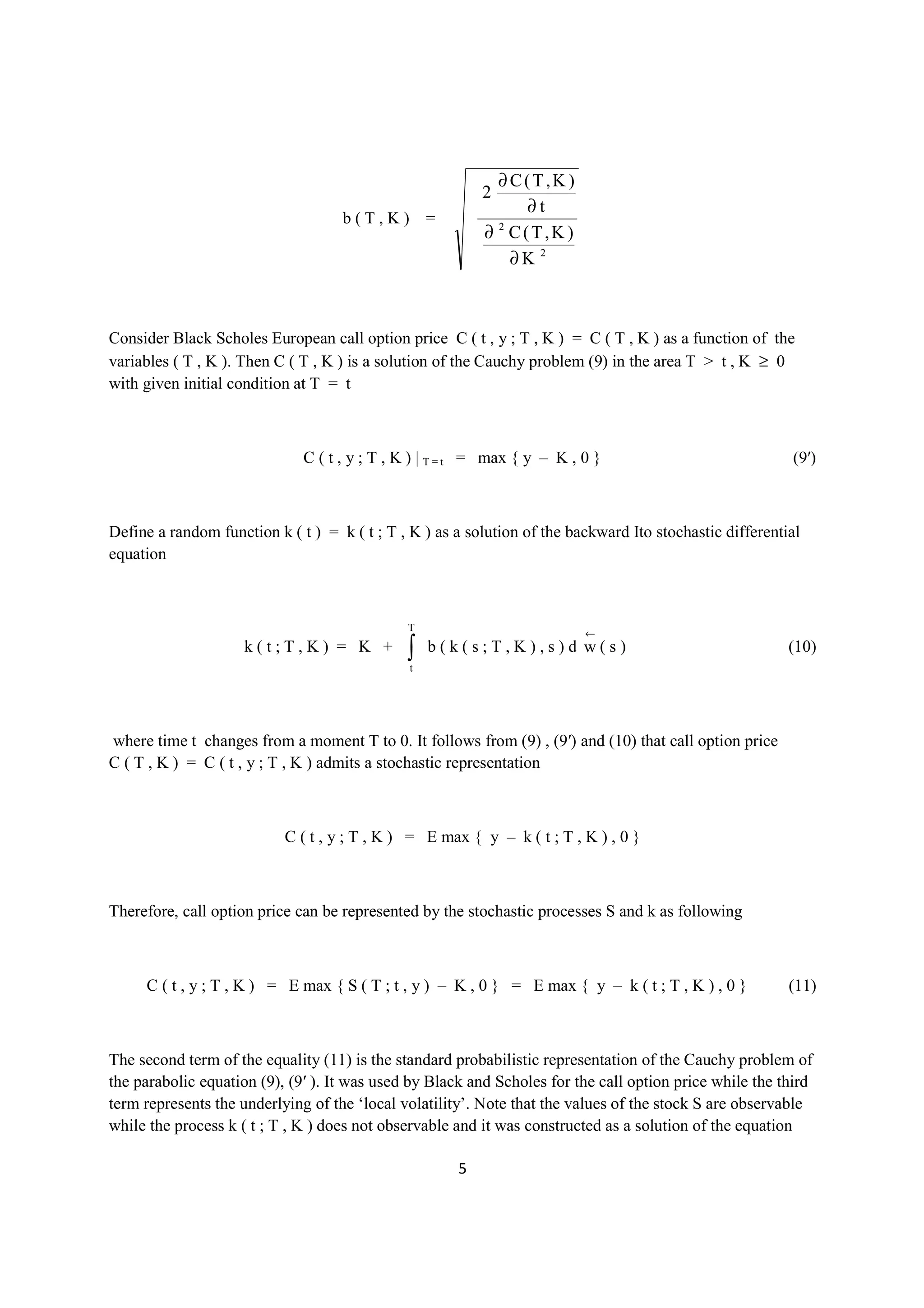
price C ( T , K ) = C ( t , y ; T , K ) is defined as
2

3. C ( t , y ; T , K ) = E max { S ( T ; t , y ) – K , 0 }
This formula admits representation
C(T,K) = ∫ (x – K)+ f(T,x)dx (2)
Twice differentiation in (2) with respect to variable K leads to the equality
∂ 2 C(T, K)
f(T,x)|x= K = (3)
∂K 2
Let us consider a solution of the equation
d ξ ( t ) = b ( t , ξ ( t )) d W ( t ) (4)
where diffusion coefficient b ( t , x ) ≥ δ 2 > 0 is unknown function. The Fokker-Planck
( first Kolmogorov) equation for the density f ( t , x ) is
∂2 ∂f
(b 2 f ) = (5)
∂x 2
∂t
Bearing in mind equality (3) and changing the order of derivatives in (5) we arrive at the equation
∂2 2 ∂ C ∂ 2 ∂C
2
(b ) =
∂ x2 ∂ x2 ∂ x2 ∂ t
3

4. ∂C
Assume that lim = 0. Then twice integration in x of the latter equation leads to the equation
x→+∞ ∂t
1 2 ∂2C ∂C
b = (6)
2 ∂x 2
∂t
Solving equation (6) for b we have
∂ C( t,x )
2
∂t
b(t,x) = (7)
∂ C( t,x )
2
∂ x2
Compare (1) and (4) we see that
xσ(x,t) = b(x,t) (8)
Reminding that variables ( t , x ) are used for ( T , K ) we can rewrite (5) in the form
1 2 ∂2 C ∂C
b (K,T) = (9)
2 ∂ K2 ∂T
This equation has the same type as the classical Black Scholes Equation.
Comment. Consider an European call option price at the date t given that the value of underlying at t is
equal to y. Denote C ( t , y ; T , K ) the Black Scholes call option price at date t. Recall that the
coordinate space of the local volatility diffusion is the space ( T , K ) and define diffusion coefficient
b ( T , K ) by the formula (7)
4

5. ∂C(T,K )
2
∂t
b(T,K) =
∂ C(T,K )
2
∂K 2
Consider Black Scholes European call option price C ( t , y ; T , K ) = C ( T , K ) as a function of the
variables ( T , K ). Then C ( T , K ) is a solution of the Cauchy problem (9) in the area T > t , K ≥ 0
with given initial condition at T = t
C ( t , y ; T , K ) | T = t = max { y – K , 0 } (9′)
Define a random function k ( t ) = k ( t ; T , K ) as a solution of the backward Ito stochastic differential
equation
T
←
k(t;T,K) = K + ∫t
b(k(s;T,K),s)d w(s) (10)
where time t changes from a moment T to 0. It follows from (9) , (9′) and (10) that call option price
C ( T , K ) = C ( t , y ; T , K ) admits a stochastic representation
C ( t , y ; T , K ) = E max { y – k ( t ; T , K ) , 0 }
Therefore, call option price can be represented by the stochastic processes S and k as following
C ( t , y ; T , K ) = E max { S ( T ; t , y ) – K , 0 } = E max { y – k ( t ; T , K ) , 0 } (11)
The second term of the equality (11) is the standard probabilistic representation of the Cauchy problem of
the parabolic equation (9), (9′ ). It was used by Black and Scholes for the call option price while the third
term represents the underlying of the ‘local volatility’. Note that the values of the stock S are observable
while the process k ( t ; T , K ) does not observable and it was constructed as a solution of the equation
5

6. (10). This auxiliary process k ( t ; T , K ) by no means does not generalize the security S ( T ; t , y ). These
two stochastic processes are different and are defined on the different coordinate spaces. It looks as an
error an attempt to replace real stock equation by the virtual stochastic process (10). This remark has dealt
with the formal implementation of the local volatility concept. On the other hand one can highlight logical
background of the local volatility concept.
The primary idea of the ‘local volatility’ is transformation of the stochastic process (1) in the
generalized form (1′′), (4). This generalized form of the stock price intends to eliminate the discrepancy
between real asset volatility and volatility implied by the option prices. One can see that implementation
of this idea the initial condition (9′) was ignored. Ignoring (9′) we lost the subordinated connection
between two pairs of variables y , t and T , K . Missing the condition (9′) one can consider T , K as free
variables and we can change notation of the pair T , K to t , y. Then we arrive at stock price governed by
the non-linear Ito equation with diffusion coefficient b ( y , t ). As far as underlying stock effects on call
option pricing through its coefficient b ( y , t ) the Black Scholes equation would be replaced by (6) which
is defined in the domain t ∈ [ 0 , T ) , y > 0 with the boundary condition that reflects European call
payoff C ( T , y ; T , K ) = max { y – K , 0 }. Now note that starting with b ( t , y ) we can construct
b ( 2 ) ( T , K ) which would be defined by the formula (7) where call option price on the right hand side (7)
is the BS price having underlying with volatility b ( t , x ). On the other hand one can remark that
coordinate space of the process (1′′) is x, x > 0. The call option function (2) uses x as well as the other
independent variable K. The attempt in (9) to replace variable x by K looks incorrect. Indeed, variable x is
initially was chosen for S. If we assume that K can be chosen for coordinate space of the process S then
one need to use other independent variable for the strike price. These two independent variables becomes
bounded by the definition of call option price C. From this moment x cannot be replaced by K. This is
essence of the free and bounded variables.
The local volatility concept was developed based on Black Scholes option pricing. It might be
make sense a brief comment the benchmark pricing too. Recall that Black Scholes option pricing is
defined by the formula
C ( T , y ; T , K ) = exp – r ( T – t ) E max { S r ( T ; t , y ) – K , 0 } (12)
where S r ( T ; t , y ) is so-called risk-neutral stock price which follows the SDE
dSr(t) = rSr(t)dt + σSr(t)dw(t)
where r ≥ 0 is a constant risk-free rate. The real stock price is assumed to be governed by the equation
dS(t) = µS(t)dt + σS(t)dw(t)
6

7. Here µ is a constant expected real return and two random processes S r ( t ) , S ( t ) are defined on initial
probability space { Ω , F , P } that in financial applications is referred to as the real world. These two
processes have equal diffusion coefficients and therefore the measures associated with these processes are
absolutely continuous. This fact gives a possibility to establish connection between real and neutral
worlds by assuming that the real process S ( t ) is defined on the other probability space { Ω , F , Q }
which usually called risk neutral world. Measure Q is chosen such that the finite distributions of the
process S ( t ) with respect to Q coincides with the correspondent distributions of the process S r ( t ) with
respect to measure P. Note that this interpretation does not make sense as far as the stock price S ( t ) is
initially were defined on the real world { Ω , F , P } regardless whether options are existed or not.
Therefore, the risk neutral world leads us to a contradiction between financial sense of a stock stochastic
model and the heuristic connection between virtual process S r ( t ) that was used by Black and Scholes
for their derivatives pricing concept. Actually we do not need to use risk neutral world. More correctly is
to say that the real underlying of the BS pricing is the process S r ( t ) which replaces the real stock S ( t ).
Black and Scholes pricing is also closely related to arbitrage free concept. The arbitrage free
concept is based on assumption that the ‘fair’ or ’perfect’ derivatives price at the current moment is a
deterministic value. Indeed, in this case the equality of the expected present value, EPV lead us to the
formula (12). Recall that EPV concept is the primary concept of the modern finance theory used to justify
the equality of two arbitrary cash flows. The pricing based on equality of two EPVs is called arbitrage
free pricing. This is why BS pricing has been referred to as arbitrage free.
There exists another approach to determine equality of two cash flows. It is the pathwise equality
of the rates of return. This concept admits equality of the rates of return for each scenario and can be
shortly outlined as following. We call two investments are equal on [ 0 , T ] if their rates of return are
equal for each scenario ω ∈ Ω for any t ∈ [ 0 , T ]. Applying this principle for pricing of a European call
option we can write the equation
S( T; t , y ) max { S ( T ; t , y ) − K , 0 }
χ{S(T;t,y) > K} =
y C( t , y ; T, K )
0 ≤ t ≤ T. This equation suggests equal rate of return on the real stock and its call option for each
scenario over an interval [ t , T ]. On the other hand we suppose that the call option price at t is equal to 0
for any scenario ω ∈ Ω such that S ( T, ω ) ≤ K. This pricing is indeed represents the perfect replication.
The stochastic price C ( t , y ; T , K ; ω ) forms the market of the call option while the market spot price
c ( t , y ; T , K ) at date t of the call option can be modeled by different ways. One way to define spot
price is for example
c(t,y; T,K) = a(t)E{C(t,y ; T,K)|Ft} + q(t)
7

8. Here F t denotes the minimal σ-algebra generating by the values of the real underlying stock on [ t , T ]
where a ( t ) , q ( t ) are deterministic or F t – measurable functions. In more general scheme one can
assume that spot price c ( t ) = c ( t , y ; T , K ) is F t – measurable function defined by SDE in the
form
t
c(t,y; T,K) = c(0) + ∫
0
a(s)E{C(s,y;T,K)|Fs}ds +
t
+ ∫
0
q(s)E{C(s,y;T,K)|Fs}dw(s)
where parameters of the problem c ( 0 ), a ( s ), q ( s ) have to be found from observations of historical
option prices.
8

9. References.
1. Dupire, B., Pricing and Hedging with Smiles , Research paper, 1993, p.9.
2. Dupire, B., Pricing with a Smile , Risk Magazine, 7, 1994, p.8 - 20.
3. Derman, E. and I. Kani (1994). Riding On A Smile, RISK, 7 (February), p.32-39.
4. Gikhman, I., Remark on Local Volatility,
http://papers.ssrn.com/sol3/papers.cfm?abstract_id=1270153, September 18, 2008.
5. Carr, P., FAQ’s in Option Pricing Theory,
http://www.math.nyu.edu/research/carrp/papers/pdf/faq2.pdf, 2002.
9