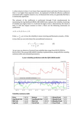
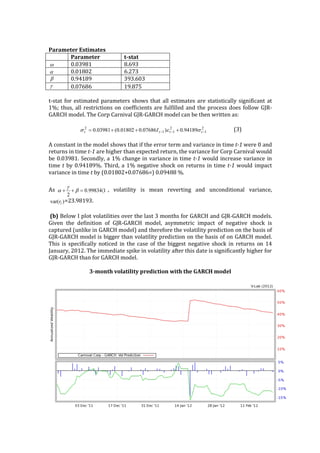
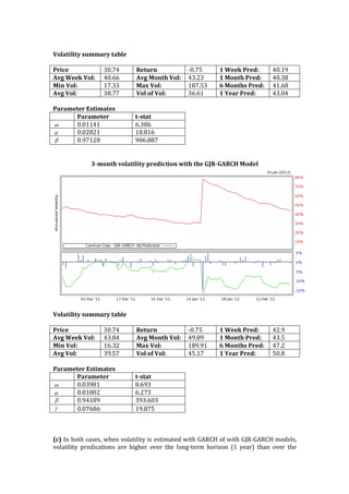
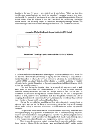
The document discusses asymmetric volatility, primarily focusing on the GJR-GARCH model, which accounts for increased volatility during market downturns compared to upturns. It compares volatility predictions using GARCH and GJR-GARCH models, highlighting the significance of capturing negative shocks for variance analysis. Additionally, it addresses short-term versus long-term volatility assessments and the relevance of implied volatility in risk management, particularly during financial crises.

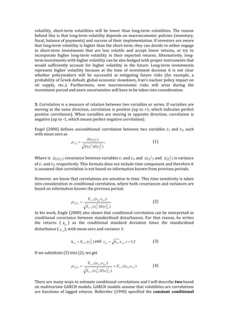
![correlation
(CCC)
multivariate
GARCH
specification,
where
conditional
covariances
and
variances
are
time-‐‑varying,
but
conditional
correlations
are
constant.
Conditional
variances
are
modelled
by
univariate
GARCH
models
and
correlation
matrix
is
estimated
by
MLE.
The
assumption
of
constant
correlations
allows
for
comparison
between
periods.
The
model
is
described
as
follows.
The
multivariate
GARCH
assumes
that
distribution
of
returns
(rt)
from
n
assets
has
mean
zero
and
covariance
matrix
Ht
(Engle,
Sheppard,
2001):
,
(5)
where
,
and
Conditional
covariance
matrix
Ht
is
then
decomposed
into
nxn
Rt
matrix
m
where
(6)
and
D
is
conditional
correlation
matrix
with
constant
correlations,
= ;
,
where
,
i=1,
…N.
Thus,
the
time
variation
in
covariance
matrix
Ht
is
then
explained
only
by
time-‐‑varying
conditional
variances
for
all
rt.
The
off-‐‑diagonal
elements
of
the
conditional
covariance
matrix
can
be
then
written
as
(Silvennoinen,
Terasvirta,
2008)
,
and
(7)
While
the
advantage
of
this
model
is
that
is
easy
to
estimate
(we
only
need
non
linear
n
estimates
of
univariate
GARCH
models),
the
problem
is
that
correlations
are
not
always
constant.
Engle
(2000,
2001)
therefore
suggested
an
alternative
estimation
of
conditional
correlations
with
dynamic
conditional
correlation
(DCC)
multivariate
GARCH
specification,
which
is
derived
from
Bollerslev’s
CCC
model,
but
allows
for
conditional
correlations
to
be
time-‐‑varying.
The
conditional
covariance
matrix
is
then
written
as
(8)
Conditional
correlations
are
then
estimated
on
the
basis
of
exponential
smoothing:
,
(9)
where
smoothing
is
introduced
through
),0( tt HNr »
ttt DRRH =
[ ]ijtt hH =
{ }tit hdiagR ,=
ijtr ijr [ ]ijD r=
1=iir
[ ] ijjtitijt hhH r= ji ¹ Nji ££ ,1
tttt RDRH =
[ ] jit
stj
s
s
sti
s
s
s
stjsti
s
tji R ,
2
,
1
2
,
1
1
,,
,, =
÷
÷
ø
ö
ç
ç
è
æ
÷
÷
ø
ö
ç
ç
è
æ
=
-
¥
=
-
¥
=
¥
=
--
åå
å
elel
eel
r](https://image.slidesharecdn.com/topicsvolatility-181129134313/85/Topics-Volatility-7-320.jpg)