Chapter 2 focuses on the econometrics of high frequency data, aimed at those interested in finance, statistics, and econometrics. It introduces the probabilistic models for high frequency data and emphasizes estimating volatility, applicable to various financial analysis methods. The document discusses methodologies for estimation, variations in literature, and the implications for risk management and financial forecasting.
![110 THE ECONOMETRICS OF HIGH FREQUENCY DATA
Andersen and Bollerslev (1998), Andersen, Bollerslev, Diebold, and Labys
(2001, 2003), Andersen, Bollerslev, and Meddahi (2005), Dacorogna, Gençay,
Müller, Olsen, and Pictet (2001), and Meddahi (2001). Methodologies based
on high frequency data can also be found in neural science (see, for example,
Valdés-Sosa, Bornot-Sánchez, Melie-Garcı́a, Lage-Castellanos, and Canales-
Rodriguez (2007)) and climatology (see Ditlevsen, Ditlevsen and Andersen
(2002) and Ditlevsen and Sørensen (2004) on Greenlandic ice cores).
The purpose of this article, however, is not so much to focus on the applica-
tions as on the probabilistic setting and the estimation methods. The theory was
started, on the probabilistic side, by Jacod (1994) and Jacod and Protter (1998),
and on the econometric side by Foster and Nelson (1996) and Comte and Re-
nault (1998). The econometrics of integrated volatility was pioneered in An-
dersen et al. (2001, 2003), Barndorff-Nielsen and Shephard (2002, 2004b) and
Dacorogna et al. (2001). The authors of this article started to work in the area
through Zhang (2001), Zhang, Mykland, and Aı̈t-Sahalia (2005), and Mykland
and Zhang (2006). For further references, see Section 2.5.5.
Parametric estimation for discrete observations in a fixed time interval is also
an active field. This problem has been studied by Genon-Catalot and Jacod
(1994), Genon-Catalot, Jeantheau, and Larédo (1999; 2000), Gloter (2000),
Gloter and Jacod (2001b, 2001a), Barndorff-Nielsen and Shephard (2001),
Bibby, Jacobsen, and Sørensen (2009), Elerian, Siddhartha, and Shephard
(2001), Jacobsen (2001), Sørensen (2001), and Hoffmann (2002). This is, of
course, only a small sample of the literature available. Also, these references
only concern the type of asymptotics considered in this paper, where the sam-
pling interval is [0, T]. There is also a substantial literature on the case where
T → ∞ (see Section 1.2 of Mykland (2010b) for some of the main references
in this area).
This article is meant to be a moderately self-contained course on the basics of
this material. The introduction assumes some degree of statistics/econometric
literacy, but at a lower level than the standard probability text. Some of the
material is research front and not published elsewhere. This is not meant as a
full review of the area. Readers with a good probabilistic background can skip
most of Section 2.2, and occasional other sections.
The text also mostly overlooks (except Sections 2.3.5 and 2.6.3) the questions
that arise in connection with multidimensional processes. For further litera-
ture in this area, one should consult Barndorff-Nielsen and Shephard (2004a),
Hayashi and Yoshida (2005) and Zhang (2011).](https://image.slidesharecdn.com/i-241105032402-0ece1b19/85/I-A-1-Econometrics_of_High_Frequency_Data-pdf-2-320.jpg)

![TIME VARYING DRIFT AND VOLATILITY 117
Microstructure Noise
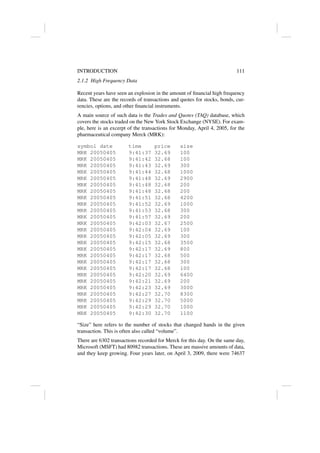
An important feature of actual transaction prices is the existence of microstruc-
ture noise. Transaction prices, as actually observed, are typically best modeled
on the form Yt = log St = the logarithm of the stock price St at time t, where
for transaction at time ti,
Yti
= Xti
+ noise,
and Xt is a semimartingale. This is often called the hidden semimartingale
model. This issue is an important part of our narrative, and is further discussed
in Section 2.5, see also Section 2.6.4.
Unequally Spaced Observations
In the above, we assumed that the transaction times ti are equally spaced. A
quick glance at the data snippet in Section 2.1.2 reveal that this is typically not
the case. This leads to questions that will be addressed as we go along.
2.1.8 A Note on Probability Theory, and other Supporting Material
We will extensively use probability theory in these notes. To avoid making a
long introduction on stochastic processes, we will define concepts as we need
them, but not always in the greatest depth. We will also omit other concepts
and many basic proofs. As a compromise between the rigorous and the in-
tuitive, we follow the following convention: the notes will (except when the
opposite is clearly stated) use mathematical terms as they are defined in Jacod
and Shiryaev (2003). Thus, in case of doubt, this work can be consulted.
Other recommended reference books on stochastic process theory are Karatzas
and Shreve (1991), Øksendal (2003), Protter (2004), and Shreve (2004). For in-
troduction to measure theoretic probability, one can consult Billingsley (1995).
Mardia, Kent, and Bibby (1979) provides a handy reference on normal distri-
bution theory.
2.2 A More General Model: Time Varying Drift and Volatility
2.2.1 Stochastic Integrals, Itô-Processes
We here make some basic definitions. We consider a process Xt, where the
time variable t ∈ [0, T]. We mainly develop the univariate case here.](https://image.slidesharecdn.com/i-241105032402-0ece1b19/85/I-A-1-Econometrics_of_High_Frequency_Data-pdf-9-320.jpg)
![118 THE ECONOMETRICS OF HIGH FREQUENCY DATA
Information Sets, σ-fields, Filtrations
Information is usually described with so-called σ-fields. The setup is as fol-
lows. Our basic space is (Ω, F), where Ω is the set of all possible outcomes
ω, and F is the collection of subsets A ⊆ Ω that will eventually be decidable
(it will be observed whether they occured or not). All random variables are
thought to be a function of the basic outcome ω ∈ Ω.
We assume that F is a so-called σ-field. In general,
Definition 2.2 A collection A of subsets of Ω is a σ-field if
(i) ∅, Ω ∈ A;
(ii) if A ∈ A, then Ac
= Ω − A ∈ A; and
(iii) if An, n = 1, 2, ... are all in A, then ∪∞
n=1An ∈ A.
If one thinks of A as a collection of decidable sets, then the interpretation of
this definition is as follows:
(i) ∅, Ω are decidable (∅ didn’t occur, Ω did);
(ii) if A is decidable, so is the complement Ac
(if A occurs, then Ac
does not
occur, and vice versa);
(iii) if all the An are decidable, then so is the event ∪∞
n=1An (the union occurs
if and only if at least one of the Ai occurs).
A random variable X is called A-measurable if the value of X can be decided
on the basis of the information in A. Formally, the requirement is that for all
x, the set {X ≤ x} = {ω ∈ Ω : X(ω) ≤ x} be decidable (∈ A).
The evolution of knowledge in our system is described by the filtration (or
sequence of σ-fields) Ft, 0 ≤ t ≤ T. Here Ft is the knowledge available at
time t. Since increasing time makes more sets decidable, the family (Ft) is
taken to satisfy that if s ≤ t, then Fs ⊆ Ft.
Most processes will be taken to be adapted to (Ft): (Xt) is adapted to (Ft)
if for all t ∈ [0, T], Xt is Ft-measurable. A vector process is adapted if each
component is adapted.
We define the filtration (FX
t ) generated by the process (Xt) as the smallest
filtration to which Xt is adapted. By this we mean that for any filtration F0
t to
which (Xt) is adapted, FX
t ⊆ F0
t for all t. (Proving the existence of such a
filtration is left as an exercise for the reader).
Wiener Processes
A Wiener process is Brownian motion relative to a filtration. Specifically,](https://image.slidesharecdn.com/i-241105032402-0ece1b19/85/I-A-1-Econometrics_of_High_Frequency_Data-pdf-10-320.jpg)
![TIME VARYING DRIFT AND VOLATILITY 119
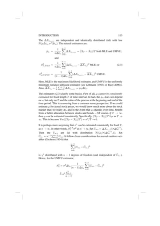
Definition 2.3 The process (Wt)0≤t≤T is an (Ft)-Wiener process if it is adpted
to (Ft) and
(1) W0 = 0;
(2) t → Wt is a continuous function of t;
(3) W has independent increments relative to the filtration (Ft): if t s, then
Wt − Ws is independent of Fs;
(4) for t s, Wt −Ws is normal with mean zero and variance t−s (N(0,t-s)).
Note that a Brownian motion (Wt) is an (FW
t )-Wiener process.
Predictable Processes
For defining stochastic integrals, we need the concept of predictable process.
“Predictable” here means that one can forecast the value over infinitesimal time
intervals. The most basic example would be a “simple process”. This is given
by considering break points 0 = s0 = t0 ≤ s1 t1 ≤ s2 t2 ... ≤ sn
tn ≤ T, and random variables H(i)
, observable (measurable) with respect to
Fsi
.
Ht =
H(0)
if t = 0
H(i)
if si t ≤ ti
(2.5)
In this case, at any time t (the beginning time t = 0 is treated separately), the
value of Ht is known before time t.
Definition 2.4 More generally, a process Ht is predictable if it can be written
as a limit of simple functions H
(n)
t . This means that H
(n)
t (ω) → Ht(ω) as
n → ∞, for all (t, ω) ∈ [0, T] × Ω.
All adapted continuous processes are predictable. More generally, this is also
true for adapted processes that are left continuous (càg, for continue à gauche).
(Proposition I.2.6 (p. 17) in Jacod and Shiryaev (2003)).
Stochastic Integrals
We here consider the meaning of the expression
Z T
0
HtdXt. (2.6)
The ingredients are the integrand Ht, which is assumed to be predictable, and
the integrator Xt, which will generally be a semi-martingale (to be defined
below in Section 2.2.3).
The expression (2.6) is defined for simple process integrands as
X
i
H(i)
(Xti
− Xsi
). (2.7)](https://image.slidesharecdn.com/i-241105032402-0ece1b19/85/I-A-1-Econometrics_of_High_Frequency_Data-pdf-11-320.jpg)
![TIME VARYING DRIFT AND VOLATILITY 123
For further details and proof of theorem, see Section 34 (p. 445-455) of Billings-
ley (1995).
This way of defining conditional expectation is a little counterintuitive if un-
familiar. In particular, the conditional expectation is a random variable. The
heuristic is as follows. Suppose that Y is a random variable, and that A car-
ries the information in Y . Introductory textbooks often introduce conditional
expectation as a non-random quantity E(X|Y = y). To make the connection,
set
f(y) = E(X|Y = y).
The conditional expectation we have just defined then satisfies
E(X|A) = f(Y ). (2.11)
The expression in (2.11) is often written E(X|Y ).
Properties of Conditional Expectations
• Linearity: for constant c1, c2:
E(c1X1 + c2X2 | A) = c1E(X1 | A) + c2E(X2 | A)
• Conditional constants: if Z is A-measurable, then
E(ZX|A) = ZE(X|A)
• Law of iterated expectations (iterated conditioning, Tower property): if A0
⊆
A, then
E[E(X|A)|A0
] = E(X|A0
)
• Independence: if X is independent of A:
E(X|A) = E(X)
• Jensen’s inequality: if g : x → g(x) is convex:
E(g(X)|A) ≥ g(E(X|A))
Note: g is convex if g(ax + (1 − a)y) ≤ ag(x) + (1 − a)g(y) for 0 ≤ a ≤ 1.
For example: g(x) = ex
, g(x) = (x − K)+
. Or g00
exists and is continuous,
and g00
(x) ≥ 0.
Martingales
An (Ft) adapted process Mt is called a martingale if E|Mt| ∞, and if, for
all s t,
E(Mt|Fs) = Ms.](https://image.slidesharecdn.com/i-241105032402-0ece1b19/85/I-A-1-Econometrics_of_High_Frequency_Data-pdf-15-320.jpg)
![124 THE ECONOMETRICS OF HIGH FREQUENCY DATA
This is a central concept in our narrative. A martingale is also known as a fair
game, for the following reason. In a gambling situation, if Ms is the amount of
money the gambler has at time s, then the gambler’s expected wealth at time
t s is also Ms. (The concept of martingale applies equally to discrete and
continuous time axis).
Example 2.6 A Wiener process is a martingale. To see this, for t s, since
Wt − Ws is N(0,t-s) given Fs, we get that
E(Wt|Fs) = E(Wt − Ws|Fs) + Ws
= E(Wt − Ws) + Ws by independence
= Ws.
A useful fact about martingales is the representation by final value: Mt is a
martingale for 0 ≤ t ≤ T if and only if one can write (with E|X| ∞)
Mt = E(X|Ft) for all t ∈ [0, T]
(only if by definition (X = MT ), if by Tower property). Note that for T =
∞ (which we do not consider here), this property may not hold. (For a full
discussion, see Chapter 1.3.B (p. 17-19) of Karatzas and Shreve (1991)).
Example 2.7 If Ht is a bounded predictable process, then for any martingale
Xt,
Mt =
Z t
0
HsdXs
is a martingale. To see this, consider first a simple process (2.5), for which
Hs = H(i)
when si s ≤ ti. For given t, if si t, by the properties of
conditional expectations,
E
H(i)
(Xti
− Xsi
)|Ft
= E
E(H(i)
(Xti
− Xsi
)|Fsi
)|Ft
= E
H(i)
E(Xti
− Xsi
|Fsi
)|Ft
= 0,
and similarly, if si ≤ t ≤ ti, then
E
H(i)
(Xti
− Xsi
)|Ft
= H(i)
(Xt − Xsi
)
so that
E(MT |Ft) = E
X
i
H(i)
(Xti
− Xsi
)|Ft
!
=
X
i:tit
H(i)
(Xti
− Xsi
) + I{ti ≤ t ≤ si}H(i)
(Xt − Xsi
)
= Mt.](https://image.slidesharecdn.com/i-241105032402-0ece1b19/85/I-A-1-Econometrics_of_High_Frequency_Data-pdf-16-320.jpg)
![TIME VARYING DRIFT AND VOLATILITY 127
where the supremum is over all grids 0 = t0 t1 ... tn = T, and all n.
In particular, an Itô process is a semimartingale, with
Mt =
Z t
0
σsdWs and
At =
Z t
0
µsds.
A supermartingale is semimartingale for which At is nonincreasing. A sub-
martingale is a semimartingale for which At is nondecreasing.
2.2.4 Quadratic Variation of a Semimartingale
Definitions
We start with some notation. A grid of observation times is given by
G = {t0, t1, ..., tn},
where we suppose that
0 = t0 t1 ... tn = T.
Set
∆(G) = max
1≤i≤n
(ti − ti−1).
For any process X, we define its quadratic variation relative to grid G by
[X, X]G
t =
X
ti+1≤t
(Xti+1
− Xti
)2
. (2.15)
We note that the quadratic variation is path-dependent. One can more generally
define the quadratic covariation
[X, Y ]G
t =
X
ti+1≤t
(Xti+1
− Xti
)(Yti+1
− Yti
).
An important theorem of stochastic calculus now says that
Theorem 2.10 For any semimartingale, there is a process [X, Y ]t so that
[X, Y ]G
t
p
→[X, Y ]t for all t ∈ [0, T], as ∆(G) → 0.
The limit is independent of the sequence of grids G.
The result follows from Theorem I.4.47 (p. 52) in Jacod and Shiryaev (2003).
The ti can even be stopping times.](https://image.slidesharecdn.com/i-241105032402-0ece1b19/85/I-A-1-Econometrics_of_High_Frequency_Data-pdf-19-320.jpg)
![128 THE ECONOMETRICS OF HIGH FREQUENCY DATA
For an Itô process,
[X, X]t =
Z t
0
σ2
s ds. (2.16)
(Cf Thm I.4.52 (p. 55) and I.4.40(d) (p. 48) of Jacod and Shiryaev (2003)). In
particular, for a Wiener process W, [W, W]t =
R t
0 1ds = t .
The process [X, X]t is usually referred to as the quadratic variation of the
semimartingale (Xt). This is an important concept, as seen in Section 2.2.2.
The theorem asserts that this quantity can be estimated consistently from data.
Properties
Important properties are as follows:
(1) Bilinearity: [X, Y ]t is linear in each of X and Y : so for example, [aX +
bZ, Y ]t = a[X, Y ]t + b[Z, Y ]t.
(2) If (Wt) and (Bt) are two independent Wiener processes, then
[W, B]t = 0.
Example 2.11 For the Heston model in Section 2.2.2, one gets from first prin-
ciples that
[W, Z]t = ρ[W, W]t + (1 − ρ2
)1/2
[W, B]t
= ρt,
since [W, W]t = t and [W, B]t = 0.
(3) For stochastic integrals over Itô processes Xt and Yt,
Ut =
Z t
0
HsdXs and Vt =
Z t
0
KsdYs,
then
[U, V ]t =
Z t
0
HsKsd[X, Y ]s.
This is often written on “differential form” as
d[U, V ]t = HtKtd[X, Y ]t.
by invoking the same results that led to (2.16). For a rigorous statement, see
Property I.4.54 (p.55) of Jacod and Shiryaev (2003).
(4) For any Itô process X, [X, t] = 0.
Example 2.12 (Leverage Effect in the Heston model).
d[X, σ2
] = γσ2
t d[W, Z]t
= γσ2
ρdt.](https://image.slidesharecdn.com/i-241105032402-0ece1b19/85/I-A-1-Econometrics_of_High_Frequency_Data-pdf-20-320.jpg)
![TIME VARYING DRIFT AND VOLATILITY 129
(5) Invariance under discounting by the short term interest rate. Discounting is
important in finance theory. The typical discount rate is the risk free short term
interest rate rt. Recall that St = exp{Xt}. The discounted stock price is then
given by
S∗
t = exp{−
Z t
0
rsds}St.
The corresponding process on the log scale is X∗
t = Xt −
R t
0 rsds, so that if
Xt is given by (2.9), then
dX∗
t = (µt − rt)dt + σtdWt.
The quadratic variation of X∗
t is therefore the same as for Xt.
It should be emphasized that while this result remains true for certain other
types of discounting (such as those incorporating cost-of-carry), it is not true
for many other relevant types of discounting. For example, if one discounts by
the zero coupon bond Λt maturing at time T, the discounted log price becomes
X∗
t = Xt − log Λt. Since the zero coupon bond will itself have volatility, we
get
[X∗
, X∗
]t = [X, X]t + [log Λ, log Λ]t − 2[X, log Λ]t.
Variance and Quadratic Variation
Quadratic variation has a representation in terms of variance. The main result
concerns martingales. For E(X2
) ∞, define the conditional variance by
Var(X|A) = E((X − E(X|A))2
|A) = E(X2
|A) − E(X|A)2
and similarly Cov(X, Y |A) = E((X − E(X|A))(Y − E(Y |A)|A).
Theorem 2.13 Let Mt be a martingale, and assume that E[M, M]T ∞.
Then, for all s t,
Var(Mt|Fs) = E((Mt −Ms)2
|Fs) = E([M, M]t −[M, M]s|Fs). (2.17)
This theorem is the beginning of something important: the left hand side of
(2.17) relates to the central limit theorem, while the right hand side only con-
cerns the law of large numbers. We shall see this effect in more detail in the
sequel.
A quick argument for (2.17) is as follows. Let G = {t0, t1, ..., tn}, and let
t∗ = max{u ∈ G : u ≤ t}, and similarly for s∗. Suppose for simplicity that
s, t ∈ G. Then, for s∗ ≤ ti tj,
E((Mti+1
− Mti
)(Mtj+1
− Mtj
)|Ftj
)
= (Mti+1
− Mti
)E((Mtj+1
− Mtj
)|Ftj
)
= 0,](https://image.slidesharecdn.com/i-241105032402-0ece1b19/85/I-A-1-Econometrics_of_High_Frequency_Data-pdf-21-320.jpg)
![130 THE ECONOMETRICS OF HIGH FREQUENCY DATA
so that by the Tower rule (since Fs∗
⊆ Ftj
)
Cov(Mti+1
− Mti
, Mtj+1
− Mtj
|Fs∗
)
= E((Mti+1
− Mti
)(Mtj+1
− Mtj
)|Fs∗
)
= 0.
It follows that, for s t,
Var(Mt∗
− Ms∗
|Fs∗
) =
X
s∗≤tit∗
Var(Mti+1
− Mti
|Fs∗
)
=
X
s∗≤tit∗
E((Mti+1
− Mti
)2
|Fs∗
)
= E(
X
s∗≤tit∗
(Mti+1
− Mti
)2
|Fs∗
)
= E([M, M]G
t∗
− [M, M]G
s∗
|Fs∗
).
The result as ∆(G) → 0 then follows by uniform integrability (Theorem 25.12
(p. 338) in Billingsley (1995)).
On the basis of this, one can now show for an Itô process that
lim
h↓0
1
h
Cov(Xt+h − Xt, Yt+h − Yt|Ft) =
d
dt
[X, Y]t.
A similar result holds in the integrated sense, cf. formula (2.10). The reason
this works is that the dt terms are of smaller order than the martingale terms.
Sometimes instantaneous correlation is important. We define
cor(X, Y)t = lim
h↓0
cor(Xt+h − Xt, Yt+h − Yt|Ft),
and note that
cor(X, Y)t =
d[X, Y]t/dt
p
(d[X, X]t/dt)(d[Y, Y]t/dt)
.
We emphasize that these results only hold for Itô processes. For general semi-
martingales, one needs to involve the concept of predictable quadratic varia-
tion, cf. Section 2.2.4.
To see the importance of the instantaneous correlation, note that in the Heston
model,
cor(X, σ2
)t = ρ.
In general, if dXt = σtdWt +dt-term, and dYt = γtdBt +dt-term, where Wt
and Bt are two Wiener processes, then
cor(X, Y)t = sgn(σtγt)cor(W, B)t. (2.18)](https://image.slidesharecdn.com/i-241105032402-0ece1b19/85/I-A-1-Econometrics_of_High_Frequency_Data-pdf-22-320.jpg)
![TIME VARYING DRIFT AND VOLATILITY 131
Lévy’s Theorem
An important result is now the following:
Theorem 2.14 Suppose that Mt is a continuous (Ft)-local martingale, M0 =
0, so that [M, M]t = t. Then Mt is an (Ft)-Wiener process.
(Cf. Thm II.4.4 (p. 102) in Jacod and Shiryaev (2003)). More generally, from
properties of normal random variables, the same result follows in the vector
case: If Mt = (M
(1)
t , ..., M
(p)
t ) is a continuous (Ft)-martingale, M0 = 0,
so that [M(i)
, M(j)
]t = δijt, then Mt is a vector Wiener process. (δij is the
Kronecker delta: δij = 1 for i = j, and = 0 otherwise.)
Predictable Quadratic Variation
One can often see the symbol hX, Y it. This can be called the predictable
quadratic vartiation. Under regularity conditions, it is defined as the limit of
P
ti≤t Cov(Xti+1
− Xti
, Yti+1
− Yti
|Fti
) as ∆(G) → 0.
For Itô processes, hX, Y it = [X, Y ]t. For general semimartingales this equal-
ity does not hold. Also, except for Itô processes, hX, Y it cannot generally be
estimated consistently from data without further assumptions. For example, If
Nt is a Poisson process with intensity λ, then Mt = Nt − λt is a martin-
gale. In this case, [M, M]t = Nt (observable), while hM, Mit = λt (cannot
be estimated in finite time). For further discussion of such discontinuous pro-
cesses, see the references mentioned in Section 2.1.8, and also, in the context
of survival analysis, Andersen, Borgan, Gill, and Keiding (1992).
For continuous semimartingales, The symbol hX, Y it is commonly used in the
literature in lieu of [X, Y ]t (including in our papers).
2.2.5 Itô’s Formula for Itô processes
Main Theorem
Theorem 2.15 Suppose that f is a twice continuously differentiable function,
and that Xt is an Itô process. Then
df(Xt) = f0
(Xt)dXt +
1
2
f00
(Xt)d[X, X]t. (2.19)
Similarly, in the multivariate case, for Xt = (X
(1)
t , ..., X
(p)
t ),
df(Xt) =
p
X
i=1
∂f
∂x(i)
(Xt)dX
(i)
t +
1
2
p
X
i,j=1
∂2
f
∂x(i)∂x(j)
(Xt)d[X(i)
, X(j)
]t.](https://image.slidesharecdn.com/i-241105032402-0ece1b19/85/I-A-1-Econometrics_of_High_Frequency_Data-pdf-23-320.jpg)
![132 THE ECONOMETRICS OF HIGH FREQUENCY DATA
(Reference: Theorem I.4.57 in Jacod and Shiryaev (2003).)
We emphasize that (2.19) is the same as saying that
f(Xt) = f(X0) +
Z t
0
f0
(Xs)dXs +
1
2
Z t
0
f00
(Xs)d[X, X]s.
If we write out dXt = µtdt + σtdWt and d[X, X]t = σ2
t dt, then equation
(2.19) becomes
df(Xt) = f0
(Xt)(µtdt + σtdWt) +
1
2
f00
(Xt)σ2
t dt
= (f0
(Xt)µt +
1
2
f00
(Xt)σ2
t )dt + f0
(Xt)σtdWt.
We note, in particular, that if Xt is an Itô process, then so is f(Xt).
Example of Itô’s Formula: Stochastic Equation for a Stock Price
We have so far discussed the model for a stock on the log scale, as dXt =
µtdt + σtdWt. The price is given as St = exp(Xt). Using Itô’s formula, with
f(x) = exp(x), we get
dSt = St(µt +
1
2
σ2
t )dt + StσtdWt. (2.20)
Example of Itô’s Formula: Proof of Lévy’s Theorem (Section 2.2.4)
Take f(x) = eihx
, and go on from there. Left to the reader.
Example of Itô’s Formula: Genesis of the Leverage Effect
We here see a case where quadratic covariation between a process and it’s
volatility can arise from basic economic principles. The following is the origin
of the use of the word “leverage effect” to describe such covariation. We em-
phasize that this kind of covariation can arise from many considerations, and
will later use the term leverage effect to describe the phenomenon broadly.
Suppose that the log value of a firm is Zt, given as a GBM,
dZt = νdt + γdWt.
For simplicity, suppose that the interest rate is zero, and that the firm has bor-
rowed C dollars (or euros, yuan, ...). If there are M shares in the company, the
value of one share is therefore
St = (exp(Zt) − C)/M.](https://image.slidesharecdn.com/i-241105032402-0ece1b19/85/I-A-1-Econometrics_of_High_Frequency_Data-pdf-24-320.jpg)
![TIME VARYING DRIFT AND VOLATILITY 133
On the log scale, therefore, by Itô’s Formula,
dXt = d log(St)
=
1
St
dSt −
1
2
1
S2
t
d[S, S]t
=
M
exp(Zt) − C
dSt −
1
2
M
exp(Zt) − C
2
d[S, S]t.
Since, in the same way as for (2.20)
dSt =
1
M
d exp(Zt)
=
1
M
exp(Zt)[(ν +
1
2
γ2
)dt + γdWt].
Hence, if we set
Ut =
exp(Zt)
exp(Zt) − C
,
dXt = Ut[(ν +
1
2
γ2
)dt + γdWt] −
1
2
U2
t γ2
dt
= (νUt +
1
2
γ2
(Ut − U2
t ))dt + UtγdWt.
In other words,
dXt = µtdt + σtdWt
where
µt = νUt +
1
2
γ2
(Ut − U2
t ) and
σt = Utγ.
In this case, the log stock price and the volatility are, indeed, correlated. When
the stock price goes down, the volatility goes up (and the volatility will go to
infinity if the value of the firm approaches the borrowed amount C, since in
this case Ut → ∞. In terms of quadratic variation, the leverage effect is given
as
d[X, σ2
]t = Utγ3
d[W, U2
]t
= 2U2
t γ3
d[W, U]t since dU2
t = 2UtdUt + d[U, U]t
= −2U4
t γ4
C exp(−Zt)dt.
The last transition follows since, by taking f(x) = (1 − C exp(−x))−1
dUt = df(Zt)
= f0
(Zt)dZt + dt-terms](https://image.slidesharecdn.com/i-241105032402-0ece1b19/85/I-A-1-Econometrics_of_High_Frequency_Data-pdf-25-320.jpg)
![134 THE ECONOMETRICS OF HIGH FREQUENCY DATA
so that
d[W, U]t = f0
(Zt)d[W, Z]t
= f0
(Zt)γdt
= −U2
t C exp(−Zt)γdt,
since f0
(x) = −f(x)2
C exp(−x).
A perhaps more intuitive result is obtained from (2.18), by observing that
sgn(d[X, σ2
]t/dt) = −1: on the correlation scale, the leverage effect is
cor(X, σ2
)t = −1.
2.2.6 Nonparametric Hedging of Options
Suppose we can set the following prediction intervals at time t = 0:
R+
≥
Z T
0
rudu ≥ R−
and Ξ+
≥
Z T
0
σ2
udu ≥ Ξ−
(2.21)
Is there any sense that we can hedge an option based on this interval?
We shall see that for a European call there is a strategy, beginning with wealth
C(S0, Ξ+
, R+
), which will be solvent for the option payoff so long as the
intervals in (2.21) are realized.
First note that by direct differentiation in (2.4), one obtains the two (!!!) Black-
Scholes-Merton differential equations
1
2
CSSS2
= CΞ and − CR = C − CSS (2.22)
(recall that C(S, Ξ, R) = SΦ(d1)−K exp(−R)Φ(d2) and d1,2 = (log(S/K)
+R ± Ξ/2)/
√
Ξ).
In analogy with Section 2.1.6, consider the financial instrument with price at
time t:
Vt = C(St, Ξt, Rt),
where
Rt = R+
−
Z t
0
rudu and Ξt = Ξ+
−
Z t
0
σ2
udu.
We shall see that the instrument Vt can be self financed by holding, at each
time t,
CS(St, Ξt, Rt) units of stock, in other words StCS(St, Ξt, Rt) $ of stock, and
Vt − StCS(St, Ξt, Rt) = −CR(St, Ξt, Rt) $ in bonds. (2.23)](https://image.slidesharecdn.com/i-241105032402-0ece1b19/85/I-A-1-Econometrics_of_High_Frequency_Data-pdf-26-320.jpg)
![BEHAVIOR OF ESTIMATORS: VARIANCE 135
where the equality follows from the first equation in (2.22). Note first that,
from Itô’s formula,
dVt = dC(St, Ξt, Rt)
= CSdSt + CRdRt + CΞdΞt +
1
2
CSSd[S, S]t
= CSdSt − CRrtdt−CΞσ2
t dt +
1
2
CSSS2
t σ2
t dt
= CSdSt − CRrtdt (2.24)
because of the second equation in (2.22).
From equation (2.24), we see that holding CS units of stock, and −CR $ of
bonds at all times t does indeed produce a P/L Vt − V0, so that starting with
V0 $ yields Vt $ at time t.
From the second equation in (2.23), we also see that Vt $ is exactly the amount
needed to maintain these positions in stock and bond. Thus, Vt has a self fi-
nancing strategy.
Estimated volatility can come into this problem in two ways:
(1) In real time, to set the hedging coefficients: under discrete observation, use
Ξ̂t = Ξ+
− estimate of integrated volatility from 0 to t.
(2) As an element of a forecasting procedure, to set intervals of the form (2.21).
For further literature on this approach, consult Mykland (2000, 2003a, 2003b,
2005, 2010b). The latter paper discusses, among other things, the use of this
method for setting reserve requirements based on an exit strategy in the event
of model failure.
For other ways of using realized volatility and similar estimators in options
trading, we refer to Zhang (2001), Hayashi and Mykland (2005), Mykland and
Zhang (2008), and Zhang (2009).
2.3 Behavior of Estimators: Variance
2.3.1 The Emblematic Problem: Estimation of Volatility
In this section, we develop the tools to show convergence in high frequency
data. As example throughout, we consider the problem of estimation of volatil-
ity. (In the absence of microstructure.) This classical problem is that of es-
timating
R t
0 σ2
s ds. The standard estimator, Realized Volatility (RV), is simply
[X, X]G
t in (2.15). The estimator is consistent as ∆(G) → 0, from the very
definition of quadratic variation.](https://image.slidesharecdn.com/i-241105032402-0ece1b19/85/I-A-1-Econometrics_of_High_Frequency_Data-pdf-27-320.jpg)
![136 THE ECONOMETRICS OF HIGH FREQUENCY DATA
This raises the question of what other properties one can associate with this
estimator. For example, does the asymptotic normality continue to hold. This
is a rather complex matter, as we shall see.
There is also the question of what to do in the presence of microstructure, to
which we return in Section 2.5.
2.3.2 A Temporary Martingale Assumption
For now consider the case where
Xt = X0 +
Z t
0
σsdWs, (2.25)
i.e., Xt is a local martingale. We shall see in Section 2.4.4 that drift terms can
easily be incorporated into the analysis.
We shall also, for now, assume that σt is bounded, i.e., there is a nonrandom
σ+ so that
σ2
t ≤ σ2
+ for all t. (2.26)
This makes Xt a martingale. We shall see in Section 2.4.5 how to remove this
assumption.
2.3.3 The Error Process
On a grid G = {t0, t1, ..., tn}, we get from Itô’s formula that
(Xti+1
− Xti
)2
= 2
Z ti+1
ti
(Xs − Xti
)dXs +
Z ti+1
ti
σ2
s ds.
If we set
t∗ = max{ti ∈ G : ti ≤ t}, (2.27)
the same equation will hold with (t∗, t) replacing (ti, ti+1). Hence
Mt =
X
ti+1≤t
(Xti+1
− Xti
)2
+ (Xt − Xt∗
)2
−
Z t
0
σ2
s ds
is a local martingale on the form
Mt = 2
X
ti+1≤t
Z ti+1
ti
(Xs − Xti
)dXs + 2
Z t
t∗
(Xs − Xt∗
)dXs.
On differential form dMt = 2(Xt − Xt∗
)dXt. We shall study the behavior of
martingales such as Mt.
Of course, we only observe [X, X]G
t =
P
ti+1≤t(Xti+1
− Xti
)2
, but we shall
see next that the same results apply to this quantity. ((Xt −Xt∗
)2
is negligible.)](https://image.slidesharecdn.com/i-241105032402-0ece1b19/85/I-A-1-Econometrics_of_High_Frequency_Data-pdf-28-320.jpg)
![BEHAVIOR OF ESTIMATORS: VARIANCE 137
2.3.4 Stochastic Order Symbols
We also make use of the following notation:
Definition 2.16 (stochastic order symbols) Let Zn be a sequence of random
variables. We say that Zn = op(1) if Zn → 0 in probability, and that Zn =
op(un) if Zn/un = op(1). Similarly, we say that Zn = Op(1) – “bounded in
probability” – if for all 0, there is an M so that supn P(|Zn| M) ≤ .
There is a theorem to the effect that this is the same as saying that for every
subsequence nk, there is a further subsequence nkl
so that Znkl
converges in
law. (See Theorem 29.3 (p. 380) in Billingsley (1995)). Finally, Zn = Op(un)
if Zn/un = Op(1).
For further discusion of this notation, see the Appendix A in Pollard (1984).
(This book is out of print, but can at the time of writing be downloaded from
http://www.stat.yale.edu/∼pollard/).
To see an illustration of the usage: under (2.26), we have that
E(Xt − Xt∗
)2
= E([X, X]t − [X, X]t∗
)
= E
Z t
t∗
σ2
s ds
≤ E(t − t∗)σ2
+
≤ E∆(G)σ2
+
so that (Xt − Xt∗
)2
= Op(E∆(G)), by Chebychev’s inequality.
2.3.5 Quadratic Variation of the Error Process: Approximation by Quarticity
An Important Result
To find the variance of our estimate, we start by computing the quadratic vari-
ation
[M, M]t = 4
X
ti+1≤t
Z ti+1
ti
(Xs − Xti
)2
d[X, X]s
+ 4
Z t
t∗
(Xs − Xt∗
)2
d[X, X]s. (2.28)
It is important here that we mean [M, M]t, and not [M, M]G
t .
A nice result, originally due to Barndorff-Nielsen and Shephard (2002), con-
cerns the estimation of this variation. Define the quarticity by
[X, X, X, X]G
t =
X
ti+1≤t
(Xti+1
− Xti
)4
+ (Xt − Xt∗
)4
.](https://image.slidesharecdn.com/i-241105032402-0ece1b19/85/I-A-1-Econometrics_of_High_Frequency_Data-pdf-29-320.jpg)
![138 THE ECONOMETRICS OF HIGH FREQUENCY DATA
Use Itô’s formula to see that (where Mt is the error process from Section 2.3.3)
d(Xt − Xti
)4
= 4(Xt − Xti
)3
dXt + 6(Xt − Xti
)2
d[X, X]t
= 4(Xt − Xti
)3
dXt +
6
4
d[M, M]t,
since d[M, M]t = 4(Xt − Xti
)2
d[X, X]t. It follows that if we set
M
(2)
t =
X
ti+1≤t
Z ti+1
ti
(Xs − Xti
)3
dXs +
Z t
t∗
(Xs − Xt∗
)3
dXs
we obtain
[X, X, X, X]G
t =
3
2
[M, M]t + 4M
(2)
t .
It turns out that the M
(2)
t term is of order op(n−1
), so that (2/3)n[X, X, X, X]G
t
is a consistent estimate of the quadratic variation (2.28):
Proposition 2.17 Assume (2.26). Consider a sequence of grids Gn = {0 =
tn,0 ... tn,n = T}. Suppose that, as n → ∞, ∆(Gn) = op(1), and
n−1
X
i=0
(tn,i+1 − tn,i)3
= Op(n−2
). (2.29)
Then
sup
0≤t≤T
| [M, M]t −
2
3
[X, X, X, X]Gn
t | = op(n−1
) as n → ∞.
Note that in the following, we typically suppress the double subscript on the
times:
ti means tn,i.
The Conditions on the Times – Why They are Reasonable
Example 2.18 We first provide a simple example to emphasize that Proposi-
tion 2.17 does the right thing. Assume for simplicity that the observation times
are equidistant: ti = tn,i = iT/n, and that the volatility is constant: σt ≡ σ.
It is then easy to see that the conditions, including (2.29), are satisfied. On the
other hand, [X, X, X, X]G
t has the distribution of (T/n)2
σ4
Pn
i=1 U4
i , where
the Ui are iid standard normal. Hence, n2
3 [X, X, X, X]G
t
p
→2
3 T2
σ4
×E(N(0, 1)4
) = 2T2
σ4
. It then follows from Proposition 2.17 that n[M, M]G
t
p
→2T2
σ4
.
Example 2.19 To see more generally why (2.29) is a natural condition, con-
sider a couple of cases for the spacings.](https://image.slidesharecdn.com/i-241105032402-0ece1b19/85/I-A-1-Econometrics_of_High_Frequency_Data-pdf-30-320.jpg)
![BEHAVIOR OF ESTIMATORS: VARIANCE 139
(i) The spacings are sufficiently regular to satisfy
∆(G) = max
i
(ti+1 − ti) = Op(n−1
).
Then
n
X
i=0
(ti+1 − ti)3
≤
n
X
i=0
(ti+1 − ti)
max
i
(ti+1 − ti)
2
= T × Op(n−2
)
(ii) On the other hand, suppose that the sampling times follow a Poisson pro-
cess with parameter λ (still with t0 = 0). Denote by N the number of sampling
points in the interval [0, T], i.e., N = inf{i : ti T}. If one conditions on
N, say, N = n, the conditional distribution of the points ti, i = 1, ..., n − 1,
behave like the order statistics of n−1 uniformly distributed random variables
(see, for example, Chapter 2.3 in Ross (1996)). In other words, ti = TU(i) (for
0 i n), where U(i) is the i’th order statistic of U1, ..., Un−1, which are iid
U[0,1]. Without any asymptotic impact, now also impose tn = T (to formally
match the rest of our theory).
Now define U(0) = 0 and U(n) = 1. With these definitions, note that for i =
1, ..., n, U(i) − U(i−1) are identically distributed with the same distribution as
U(1), which has density (n − 1)(1 − x)n−2
. (See, for example, Exercise 3.67
(p. 110) in Rice (2006).) The expression in (2.29) becomes
n−1
X
i=0
(ti+1 − ti)3
= T3
n
X
i=1
(U(i) − U(i−1))3
= T3
nEU3
(1)(1 + op(1))
by the law of large numbers. Since EU3
(1) = 6
(n+1)n(n−1) = O(n−3
), (2.29)
follows.
Application to Refresh Times
We here briefly consider the case of multidimensional processes of the form
(X
(1)
t , ..., X
(p)
t ). It will often be the case that the observation occurs at asyn-
chronous times. In other words, process (X
(r)
t ) is observed at times G
(r)
n =
{0 ≤ t
(r)
n,0 t
(r)
n,1 ... t
(r)
n,nr ≤ T}, and the grids G
(r)
n are not the same.
Note that in this case, there is latitude in what meaning to assign to the symbol
n. It is an index that goes to infinity with each nr, for example n = n1+...+np.
One would normally require that nr/n is bounded away from zero.
A popular way of dealing with this problem is to use refresh times, as follows.](https://image.slidesharecdn.com/i-241105032402-0ece1b19/85/I-A-1-Econometrics_of_High_Frequency_Data-pdf-31-320.jpg)
![BEHAVIOR OF ESTIMATORS: VARIANCE 141
The Minkowski and Hölder inequalities say that
||X + Y ||p ≤ ||X||p + ||Y ||p
||XY ||1 ≤ ||X||p||Y ||q for
1
p
+
1
q
= 1.
Example 2.20 A special case of the Hölder inequalitiy is ||X||1 ≤ ||X||p
(take Y = 1). In particular, under (2.29), for for 1 ≤ v ≤ 3:
1
n
n−1
X
i=0
(ti+1 − ti)v
!1
v
≤
1
n
n−1
X
i=0
(ti+1 − ti)3
!1
3
=
1
n
× Op(n−2
)
1
3
= Op(n−3
)
1
3
= Op(n−1
),
so that
n
X
i=0
(ti+1 − ti)v
= Op(n1−v
). (2.30)
To show Proposition 2.17, we need the Burkholder-Davis-Gundy inequality
(see Section 3 of Ch. VII of Dellacherie and Meyer (1982), or p. 193 and 222
in Protter (2004)), as follows. For 1 ≤ p ∞, there are universal constants cp
and Cp so that for all continuous martingales Nt,
cp||[N, N]T ||
1/2
p/2 ≤ || sup
0≤t≤T
|Nt| ||p ≤ Cp||[N, N]T ||
1/2
p/2.
Note, in particular, that for 1 p ∞,
C2
p = qp
p(p − 1)
2
where q is given by p−1
+ q−1
= 1.
Proof of Proposition 2.17
From applying Itô’s Formula to (Xt − Xti
)8
:
[M(2)
, M(2)
]t =
X
ti+1≤t
Z ti+1
ti
(Xs − Xti
)6
d[X, X]s
+
Z t
t∗
(Xs − Xt∗
)6
d[X, X]s
=
1
28
[X; 8]G
t + martingale term
where [X; 8]G
t =
P
ti+1≤t(Xti+1
− Xti
)8
+ (Xt − Xt∗
)8
is the ochticity.](https://image.slidesharecdn.com/i-241105032402-0ece1b19/85/I-A-1-Econometrics_of_High_Frequency_Data-pdf-33-320.jpg)
![142 THE ECONOMETRICS OF HIGH FREQUENCY DATA
Note that for stopping time τ ≤ T, [X; 8]G
τ =
P
i(Xti+1∧τ − Xti∧τ )8
. Hence,
by the Burkholder-Davis-Gundy inequality (with p = 8)
E[M(2)
, M(2)
]τ =
1
28
E[X; 8]G
τ
≤
1
28
C8
8 E
X
i
([X, X]ti+1∧τ − [X, X]ti∧τ )4
≤
1
28
C8
8 σ8
+E
X
i
(ti+1 ∧ τ − ti ∧ τ)4
.
Let 0, and set
τn = inf{ t ∈ [0, T] : n2
X
i
(ti+1 ∧ t − ti ∧ t)4
}.
Then
E[M(2)
, M(2)
]τn
≤ n−2 1
28
C8
8 σ8
+. (2.31)
By assumption, n2
P
i(ti+1 ∧ t − ti ∧ t)4
≤ ∆(G)n2
P
i(ti+1 − ti)3 p
→ 0,
and hence
P(τn 6= T) → 0 as n → ∞. (2.32)
Hence, for any δ 0,
P(n sup
0≤t≤T
|M
(2)
t | δ) (2.33)
≤ P(n sup
0≤t≤τn
|M
(2)
t | δ) + P(τn 6= T)
≤
1
δ2
E
n sup
0≤t≤τn
|M
(2)
t |
2
+ P(τn 6= T) (Chebychev)
≤
1
δ2
C2
2 n2
E[M(2)
, M(2)
]τn
+ P(τn 6= T) (Burkholder-Davis-Gundy)
≤
1
δ2
C2
2
1
28
C8
8 σ8
+ + P(τn 6= T) (from (2.31))
→
1
δ2
C2
2
1
28
C8
8 σ8
+ as n → ∞ (from (2.32)).
Hence Proposition 2.17 has been shown.
2.3.7 Quadratic Variation of the Error Process: When Observation Times are
Independent of the Process
Main Approximation
We here assume that the observation times are independent of the process X.
The basic insight for the following computation is that over small intervals,](https://image.slidesharecdn.com/i-241105032402-0ece1b19/85/I-A-1-Econometrics_of_High_Frequency_Data-pdf-34-320.jpg)
![BEHAVIOR OF ESTIMATORS: VARIANCE 143
(Xt − Xt∗
)2
≈ [X, X]t − [X, X]t∗
. To the extent that this approximation is
valid, it follows from (2.28) that
[M, M]t ≈ 4
X
ti+1≤t
Z ti+1
ti
([X, X]s − [X, X]ti
)d[X, X]s
+ 4
Z t
t∗
([X, X]s − [X, X]t∗
)d[X, X]s
= 2
X
ti+1≤t
([X, X]ti+1
− [X, X]ti
)2
+ 2([X, X]t − [X, X]t∗
)2
.
We shall use this device several times in the following, and will this first time
do it rigorously.
Proposition 2.21 Assume (2.26), and that σ2
t is continuous in mean square:
sup
0≤t−s≤δ
E(σ2
t − σ2
s )2
→ 0 as δ → ∞.
Also suppose that the grids Gn are nonrandom, or independent of the process
Xt. Also suppose that, as n → ∞, ∆(G) = op(n−1/2
), and assume (2.29).
Then
[M, M]t = 2
X
ti+1≤t
([X, X]ti+1
− [X, X]ti
)2
+ 2([X, X]t − [X, X]t∗
)2
+ op(n−1
). (2.34)
If σt is continuous, it is continuous in mean square (because of (2.26)). More
generally, σt can, for example, also have Poisson jumps.
In the rest of this section, we shall write all expectations implicitly as condi-
tional on the times.
To show Proposition 2.21, we need some notation and a lemma, as follows:
Lemma 2.22 Let t∗ = max{ti ∈ G : ti ≤ t} (as in (2.27)). Let Nt be an Itô
process martingale, for which (for a, b 0), for all t,
d
dt
E[N, N]t ≤ a(t − t∗)b
.
Let Ht be a predictable process, satisfying |Ht| ≤ H+ for some constant H+.
Set
Rv(G) =
n−1
X
i=0
(ti+1 − ti)v
!
.](https://image.slidesharecdn.com/i-241105032402-0ece1b19/85/I-A-1-Econometrics_of_High_Frequency_Data-pdf-35-320.jpg)
![144 THE ECONOMETRICS OF HIGH FREQUENCY DATA
Then
||
X
ti+1≤t
Z ti+1
ti
(Ns − Nti
)Hsds +
Z t
t∗
(Ns − Nt∗
)Hsds||1
≤
H2
+
a
b + 3
Rb+3(G)
1/2
+ R(b+3)/2(G)
2
b + 3
a
b + 1
1/2
sup
0≤t−s≤∆(G)
||Hs − Ht||2.
(2.35)
Proof of Proposition 2.21. Set Nt = Mt and Ht = σ2
t . Then
d[M, M]t = 4(Xt − Xti
)2
d[X, X]t
= 4([X, X]t − [X, X]ti
)d[X, X]t + 4((Xt − Xti
)2
− ([X, X]t − [X, X]ti
))d[X, X]t
= 4([X, X]t − [X, X]ti
)d[X, X]t + 2(Nt − Nti
)σ2
t dt.
Thus, the approximation error in (2.34) is exactly of the form of the left hand
side in (2.35). We note that
Ed[N, N]t = 4E(Xt − Xti
)2
d[X, X]t
= 4E(Xt − Xti
)2
σ2
+dt
= 4(t − ti)σ4
+dt
hence the conditions of Lemma 2.22 are satisfied with a = 4σ4
+ and b = 1.
The result follows from (2.30). 2
Proof of Lemma 2.22 (Technical Material, can be omitted).
Decompose the original problem as follows:
Z ti+1
ti
(Ns − Nti
)Hsds
=
Z ti+1
ti
(Ns − Nti
)Hti
ds +
Z ti+1
ti
(Ns − Nti
)(Hs − Hti
)ds.
For the first term, from Itô’s formula, d(ti+1 − s)(Ns − Nti
) = −(Ns −
Nti
)ds + (ti+1 − s)dNs, so that
Z ti+1
ti
(Ns − Nti
)Hti
ds = Hti
Z ti+1
ti
(ti+1 − s)dNs](https://image.slidesharecdn.com/i-241105032402-0ece1b19/85/I-A-1-Econometrics_of_High_Frequency_Data-pdf-36-320.jpg)
![BEHAVIOR OF ESTIMATORS: VARIANCE 145
hence
X
ti+1≤t
Z ti+1
ti
(Ns − Nti
)Hsds
=
X
ti+1≤t
Hti
Z ti+1
ti
(ti+1 − t)dNs
+
X
ti+1≤t
Z ti+1
ti
(Ns − Nti
)(Hs − Hti
)ds. (2.36)
The first term is the end point of a martingale. For each increment,
E
Z ti+1
ti
(Ns − Nti
)Hti
ds
2
= E
Hti
Z ti+1
ti
(ti+1 − s)dNs
2
≤ H2
+E
Z ti+1
ti
(ti+1 − s)dNs
2
= H2
+E
Z ti+1
ti
(ti+1 − s)2
d[N, N]s
= H2
+
Z ti+1
ti
(ti+1 − s)2
dE[N, N]s
= H2
+
Z ti+1
ti
(ti+1 − s)2 d
ds
E[N, N]sds
= H2
+
Z ti+1
ti
(ti+1 − s)2
a(s − ti)b
ds
= H2
+
a
b + 3
(ti+1 − ti)b+3
and so, by the uncorrelatedness of martingale increments,
E
X
ti+1≤t
Hti
Z ti+1
ti
(ti+1 − t)dNs
2
≤ H2
+
a
b + 3
X
ti+1≤t
(ti+1 − ti)3
≤ H2
+
a
b + 3
Rb+3(G). (2.37)](https://image.slidesharecdn.com/i-241105032402-0ece1b19/85/I-A-1-Econometrics_of_High_Frequency_Data-pdf-37-320.jpg)
![146 THE ECONOMETRICS OF HIGH FREQUENCY DATA
On the other hand, for the second term in (2.36),
||(Ns − Nti
)(Hs − Hti
)||1
≤ ||Ns − Nti
||2||Hs − Hti
||2
≤ E(Ns − Nti
)2
1/2
||Hs − Hti
||2
= (E([N, N]s − [N, N]ti
))1/2
||Hs − Hti
||q
=
Z s
ti
d
du
E[N, N]udu
1/2
||Hs − Hti
||2
≤
Z s
ti
a(u − ti)b
du
1/2
||Hs − Hti
||2
=
a
b + 1
(s − ti)b+1
1/2
||Hs − Hti
||2
= (s − ti)(b+1)/2
a
b + 1
(s − ti)b+1
1/2
||Hs − Hti
||2,
and from this
||
Z ti+1
ti
(Ns − Nti
)(Hs − Hti
)ds||1
≤
Z ti+1
ti
||(Ns − Nti
)(Hs − Hti
)||1ds
≤
Z ti+1
ti
(s − ti)(b+1)/2
ds
a
b + 1
1/2
sup
ti≤s≤ti+1
||Hs − Hti
||2
= (ti+1 − ti)(b+3)/2 2
b + 3
a
b + 1
1/2
sup
ti≤s≤ti+1
||Hs − Hti
||2.
Hence, finally, for the second term in (2.36),
||
X
ti+1≤t
Z ti+1
ti
(Ns − Nti
)(Hs − Hti
)dt||1
≤
X
t≤ti+1
(ti+1 − ti)(b+3)/2
2
b + 3
a
b + 1
1/2
sup
0≤t−s≤∆(G)
||Hs − Ht||2
= R(b+3)/2(G)
2
b + 3
a
b + 1
1/2
sup
0≤t−s≤∆(G)
||Hs − Ht||2. (2.38)](https://image.slidesharecdn.com/i-241105032402-0ece1b19/85/I-A-1-Econometrics_of_High_Frequency_Data-pdf-38-320.jpg)
![BEHAVIOR OF ESTIMATORS: VARIANCE 147
Hence, for the overall sum (2.36), from (2.37) and (2.38) and
||
X
ti+1≤t
Z ti+1
ti
(Ns − Nti
)Hsds||1
≤ ||
X
ti+1≤t
Hti
Z ti+1
ti
(ti+1 − t)dNs||1
+ ||
X
ti+1≤t
Z ti+1
ti
(Ns − Nti
)(Hs − Hti
)ds||1
≤ ||
X
ti+1≤t
Hti
Z ti+1
ti
(ti+1 − t)dNs||2
+ ||
X
ti+1≤t
Z ti+1
ti
(Ns − Nti
)(Hs − Hti
)ds||1
≤
H2
+
a
b + 3
Rb+3(G)
1/2
+ R(b+3)/2(G)
2
b + 3
a
b + 1
1/2
sup
0≤t−s≤∆(G)
||Hs − Ht||2.
The part from t∗ to t can be included similarly, showing the result. 2
Quadratic Variation of the Error Process, and Quadratic Variation of Time
To give the final form to this quadratic variation, define the “Asymptotic Qua-
dratic Variation of Time” (AQVT), given by
Ht = lim
n→∞
n
T
X
tn,j+1≤t
(tn,j+1 − tn,j)2
, (2.39)
provided that the limit exists. From Example 2.19, we know that dividing by n
is the right order. We now get
Proposition 2.23 Assume the conditions of Proposition 2.21, and that the AQVT
exists. Then
n[M, M]t
p
→ 2T
Z t
0
σ4
s dHs.](https://image.slidesharecdn.com/i-241105032402-0ece1b19/85/I-A-1-Econometrics_of_High_Frequency_Data-pdf-39-320.jpg)
![148 THE ECONOMETRICS OF HIGH FREQUENCY DATA
The proof is a straight exercise in analysis. The heuristic for the result is as
follows. From (2.34),
[M, M]t = 2
X
ti+1≤t
([X, X]ti+1
− [X, X]ti
)2
+ 2([X, X]t − [X, X]t∗
)2
+ op(n−1
)
= 2
X
ti+1≤t
(
Z ti+1
ti
σ2
s ds)2
+ 2(
Z t
t∗
σ2
s ds)2
+ op(n−1
)
= 2
X
ti+1≤t
((ti+1 − ti)σ2
ti
)2
+ 2((t − t∗)σ2
t∗
)2
+ op(n−1
)
= 2
T
n
Z t
0
σ4
s dHs + op(n−1
).
Example 2.24 We here give a couple of examples of the AQVT:
(i) When the times are equidistant: ti+1 − ti = T/n, then
Ht ≈
n
T
X
tn,j+1≤t
T
n
2
=
T
n
#{ti+1 ≤ t}
= T × fraction of ti+1 in [0, t]
≈ T ×
t
T
= t.
(ii) When the times follow a Poisson process with parameter λ, we proceed as
in case (ii) in Example 2.19. We condition on the number of sampling points
n, and get ti = TU(i) (for 0 i n), where U(i) is the i’th order statistic of
U1, ..., Un, which are iid U[0,1]. Hence (again taking U(0) = 0 and U(n) = 1)
Ht ≈
n
T
X
tn,j+1≤t
(ti+1 − ti)2
= T2 n
T
X
tn,j+1≤t
(U(i) − U(i−1))2
= T2 n
T
X
tn,j+1≤t
EU2
(1)(1 + op(1))
= T2 n
T
#{ti+1 ≤ t}EU2
(1)(1 + op(1))
= Tn2 t
T
EU2
(1)(1 + op(1))
= 2t(1 + op(1))](https://image.slidesharecdn.com/i-241105032402-0ece1b19/85/I-A-1-Econometrics_of_High_Frequency_Data-pdf-40-320.jpg)
![BEHAVIOR OF ESTIMATORS: VARIANCE 149
by the law of large numbers, since the spacings have identical distribution, and
since EU2
(1) = 2/n(n + 1). Hence Ht = 2t.
The Quadratic Variation of Time in the General Case
We now go back to considering the times as possibly dependent with the pro-
cess X. Note that by using the Burkholder-Davis-Gundy Inequality condition-
ally, we obtain that
c4
4E(([X, X]ti+1
− [X, X]ti
)2
| Fti
)
≤ E((Xti+1
− Xti
)4
| Fti
) ≤ C4
4 E(([X, X]ti+1
− [X, X]ti
)2
| Fti
),
where c4 and C4 are as in Section 2.3.6. In the typical law of large numbers
setting, [X, X, X, X]t −
P
i E((Xti+1
− Xti
)4
| Fti
) is a martingale which is
of lower order than [X, X, X, X]t itself, and the same goes for
X
i
([X, X]ti+1
− [X, X]ti
)2
− E(([X, X]ti+1
− [X, X]ti
)2
| Fti
)
.
By the argument in Proposition 2.23, therefore, it follows that under suitable
regularity conditions, if n[X, X, X, X]t
p
→ Ut as n → ∞, and if the AQVT
Ht is absolutely continuous in t, then Ut is also absolutely continuous, and
c4
42Tσ4
t H0
t ≤ U0
t ≤ C4
4 2Tσ4
t H0
t.
This is of some theoretic interest in that it establishes the magnitude of the limit
of n[X, X, X, X]t. However, it should be noted that C4
4 = 218
/36
≈ 359.6, so
the bounds are of little practical interest.
A slightly closer analysis of this particular case uses the Bartlett type identities
for martingales to write
E((Xti+1
− Xti
)4
| Fti
)
= −3E(([X, X]ti+1
− [X, X]ti
)2
| Fti
)
+ 6E((Xti+1
− Xti
)2
([X, X]ti+1
− [X, X]ti
) | Fti
)
≤ −3E(([X, X]ti+1
− [X, X]ti
)2
| Fti
)
+ 6E((Xti+1
− Xti
)4
| Fti
)1/2
E(([X, X]ti+1
− [X, X]ti
)2
| Fti
)1/2
.
Solving this quadratic inequality yields that we can take c4
4 = (3−
√
6)2
≈ 0.3
and C4
4 = (3 +
√
6)2
≈ 29.7.
2.3.8 Quadratic Variation, Variance, and Asymptotic Normality
We shall later see that n1/2
([X, X]G
t − [X, X]t) is approximately normal. In
the simplest case, where the times are independent of the process, the nor-
mal distribution has mean zero and variance n[M, M]t ≈ 2T
R t
0 σ4
s dHs. From](https://image.slidesharecdn.com/i-241105032402-0ece1b19/85/I-A-1-Econometrics_of_High_Frequency_Data-pdf-41-320.jpg)
![150 THE ECONOMETRICS OF HIGH FREQUENCY DATA
standard central limit considerations, this is unsurprising when the σt process
is nonrandom, or more generally independent of the Wt process. (In the latter
case, one simply conditions on the σt process).
What is surprising, and requires more concepts, is that the normality result also
holds when σt process has dependence with the Wt process. For this we shall
need new concepts, to be introduced in Section 2.4.
2.4 Asymptotic Normality
2.4.1 Stable Convergence
In order to define convergence in law, we need to deal with the following is-
sue. Suppose θ̂n is an estimator of θ, say, θ̂n = [X, X]Gn
T and θ = [X, X]T =
R T
0 σ2
t dt. As suggested in Section 2.3.7, the variance of Zn = n1/2
(θ̂n − θ)
converges to 2T
R t
0 σ4
s dHs. We shall now go on to show the following conver-
gence in law:
n1/2
(θ̂n − θ)
L
→ U ×
2T
Z T
0
σ4
s dHs
1/2
,
where U is a standard normal random variable, independent of the σ2
t process.
In order to show this, we need to be able to bring along prelimiting information
into the limit: U only exists in the limit, while as argued in Section 2.3.5, the
asymptotic variance 2T
R T
0 σ4
s dHs can be estimated consistently, and so is a
limit in probability of a prelimiting quantity.
To operationalize the concept in our setting, we need the filtration (Ft) to
which all relevant processes (Xt, σt, etc) are adapted. We shall assume that
Zn (the quantity that is converging in law) to be measurable with respect to a
σ-field χ, FT ⊆ χ. The reason for this is that it is often convenient to exclude
microstructure noise from the filtration Ft. Hence, for example, the TSRV (in
Section 2.5 below) is not FT -measurable.
Definition 2.25 Let Zn be a sequence of χ-measurable random variables,
FT ⊆ χ. We say that Zn converges FT -stably in law to Z as n → ∞ if Z
is measurable with respect to an extension of χ so that for all A ∈ FT and for
all bounded continuous g, EIAg(Zn) → EIAg(Z) as n → ∞.
The definition means, up to regularity conditions, that Zn converges jointly in
law with all FT measurable random variables. This intuition will be impror-
tant in the following. For further discussion of stable convergence, see Rényi
(1963), Aldous and Eagleson (1978), Chapter 3 (p. 56) of Hall and Heyde
(1980), Rootzén (1980) and Section 2 (p. 169-170) of Jacod and Protter (1998).
We now move to the main result.](https://image.slidesharecdn.com/i-241105032402-0ece1b19/85/I-A-1-Econometrics_of_High_Frequency_Data-pdf-42-320.jpg)
![ASYMPTOTIC NORMALITY 151
2.4.2 Asymptotic Normality
We shall be concerned with a sequence of martingales Mn
t , 0 ≤ t ≤ T, n =
1, 2, ..., and how it converges to a limit Mt. We consider here only continuous
martingales, which are thought of as random variables taking values in the set
C of continuous functions [0, T] → R.
To define weak, and stable, convergence, we need a concept of continuity. We
say that g is a continuous function C → R if:
sup
0≤t≤T
|xn(t) − x(t)| → 0 implies g(xn) → g(x).
We note that if (Mn
t )
L
→ (Mt) in this process sense, then, for example, Mn
T
L
→
MT as a random variable. This is because the function x → g(x) = x(T)
is continuous. The reason for going via process convergence is (1) sometimes
this is really the result one needs, and (2) since our theory is about continuous
processes converging to a continuous process, one does not need asymptotic
negligibility conditions à la Lindeberg (these kinds of conditions are in place
in the usual CLT precisely to avoid jumps is the asymptotic process). For a re-
lated development based on discrete time predictable quadratic variations, and
Lindeberg conditions, see Theorem IX.7.28 (p. 590-591) of Jacod and Shiryaev
(2003).
In order to show results about continuous martingales, we shall use the follow-
ing assumption
Condition 2.26 There are Brownian motions W
(1)
t , ..., W
(p)
t (for some p) that
generate (Ft).
It is also possible to proceed with assumptions under which there are jumps in
some processes, but for simplicity, we omit any discussion of this here.
Under Condition 2.26, it follows from Lemma 2.1 (p. 270) in Jacod and Protter
(1998) that stable convergence in law of a local martingale Mn
to a process M
is equivalent to (straight) convergence in law of the process (W(1)
, ..., W(p)
,
Mn
) to the process (W(1)
, ..., W(p)
, M). This result does not extend to all
processes and spaces, cf. the discussion in the cited paper.
Another main fact about stable convergence is that limits and quadratic varia-
tion can be interchanged:
Proposition 2.27 (Interchangeability of limits and quadratic variation). As-
sume that Mn
is a sequence of continuous local martingales which converges
stably to a process M. Then (Mn
, [Mn
, Mn
]) converges stably to
(M, [M, M]).](https://image.slidesharecdn.com/i-241105032402-0ece1b19/85/I-A-1-Econometrics_of_High_Frequency_Data-pdf-43-320.jpg)
![152 THE ECONOMETRICS OF HIGH FREQUENCY DATA
For proof, we refer to Corollary VI.6.30 (p. 385) in Jacod and Shiryaev (2003),
which also covers the case of bounded jumps. More generally, consult ibid.,
Chapter VI.6.
We now state the main central limit theorem (CLT).
Theorem 2.28 Assume Condition 2.26. Let (Mn
t ) be a sequence of continu-
ous local martingales on [0, T], each adapted to (Ft), with Mn
0 = 0. Suppose
that there is an (Ft) adapted process ft so that
[Mn
, Mn
]t
p
→
Z t
0
f2
s ds for each t ∈ [0, T]. (2.40)
Also suppose that, for each i = 1, .., p,
[Mn
, W(i)
]t
p
→ 0 for each t ∈ [0, T]. (2.41)
There is then an extension (F0
t) of (Ft), and an (F0
t)-martingale Mt so that
(Mn
t ) converges stably to (Mt). Furthermore, there is a Brownian motion
(W0
t) so that (W
(1)
t , ..., W
(p)
t , W0
t) is an (F0
t)-Wiener process, and so that
Mt =
Z t
0
fsdW0
s. (2.42)
It is worth while to understand the proof of this result, and hence we give it
here. The proof follows more or less verbatim that of Theorem B.4 in Zhang
(2001) (p. 65-67). The latter is slightly more general.
Proof of Theorem 2.28. Since [Mn
, Mn
]t is a non-decreasing process and has
non-decreasing continuous limit, the convergence (2.40) is also in law in D(R)
by Theorem VI.3.37 (p. 354) in Jacod and Shiryaev (2003). Thus, in their ter-
minology (ibid., Definition VI.3.25, p. 351), [Mn
, Mn
]t is C-tight. From this
fact, ibid., Theorem VI.4.13 (p. 358) yields that the sequence Mn
is tight.
From this tightness, it follows that for any subsequence Mnk
, we can find a
further subsequence Mnkl which converges in law (as a process) to a limit M,
jointly with W(1)
, ..., W(p)
; in other words, (W(1)
, ..., W(p)
, Mnkl ) converges
in law to (W(1)
, ..., W(p)
, M). This M is a local martingale by ibid., Propo-
sition IX.1.17 (p. 526), using the continuity of Mn
t . Using Proposition 2.27
above, (Mnkl , [Mnkl , Mnkl ]) converge jointly in law (and jointly with the
W(i)
’s) to (M, [M, M]). From (2.40) this means that [M, M]t =
R t
0 f2
s ds. The
continuity of [M, M]t assures that Mt is continuous. By the same reasoning,
from (2.41), [M, W(i)
] ≡ 0 for each i = 1, .., p. Now let W0
t =
R t
0 f
−1/2
s dMs
(if ft is zero on a set of Lebesgue measure greater than zero, follow the alter-
native construction in Volume III of Gikhman and Skorohod (1969)). By Prop-
erty (3) in Section 2.2.4 (or refer directly to Property I.4.54 (p.55) of Jacod](https://image.slidesharecdn.com/i-241105032402-0ece1b19/85/I-A-1-Econometrics_of_High_Frequency_Data-pdf-44-320.jpg)
![ASYMPTOTIC NORMALITY 153
and Shiryaev (2003)), [W0
, W0
]t = t, while [W0
, W(i)
] ≡ 0. By the mul-
tivariate version of Lévy’s Theorem (Section 2.2.4, or refer directly to The-
orem II.4.4 (p. 102) of Jacod and Shiryaev (2003)), it therefore follows that
(W
(1)
t , ..., W
(p)
t , W0
t) is a Wiener process. The equality (2.42) follows by con-
struction of W0
t. Hence the Theorem is shown for subsequence Mnkl . Since
the subsequence Mnk
was arbitrary, Theorem 2.28 follows (cf. the Corollary
on p. 337 of Billingsley (1995)). 2
2.4.3 Application to Realized Volatility
Independent Times
We now turn our attention to the simplest application: the estimator from Sec-
tion 2.3. Consider the normalized (by
√
n) error process
Mn
t = 2n1/2
X
ti+1≤t
Z ti+1
ti
(Xs − Xti
)dXs + 2n1/2
Z t
t∗
(Xs − Xt∗
)dXs.
(2.43)
From Section 2.3.7, we have that Condition (2.40) of Theorem 2.28 is satisfied,
with
f2
t = 2Tσ4
t H0
t.
It now remains to check Condition (2.41). Note that
d[Mn
, W(i)
]t = 2n1/2
(Xt − Xt∗
)d[X, W(i)
]t.
We can now apply Lemma 2.22 with Nt = Xt and Ht = (d/dt)[X, W(i)
]t.
From the Cauchy-Schwarz inequality (in this case known as the Kunita-Wata-
nabe inequality)
|[X, W(i)
]t+h − [X, W(i)
]t|
≤
p
[X, X]t+h − [X, X]t
q
[W(i), W(i)]t+h − [W(i), W(i)]t
≤
q
σ2
+h
√
h = σ+h
(recall that the quadratic variation is a limit of sums of squares), so we can
take H+ = σ+. On the other hand, (d/dt)E[N, N]t ≤ σ2
+ = a(t − t∗)b
with
a = σ2
+ and b = 0.](https://image.slidesharecdn.com/i-241105032402-0ece1b19/85/I-A-1-Econometrics_of_High_Frequency_Data-pdf-45-320.jpg)
![154 THE ECONOMETRICS OF HIGH FREQUENCY DATA
Thus, from Lemma 2.22,
||[Mn
, W(i)
]t||1
= 2n1/2
||
X
ti+1≤t
Z ti+1
ti
(Ns − Nti
)Hsds +
Z t
t∗
(Ns − Nt∗
)Hsds||1
≤ 2n1/2
H2
+
a
b + 3
Rb+3(G)
1/2
+ R(b+3)/2(G)
2
b + 3
a
b + 1
1/2
sup
0≤t−s≤∆(G)
||Hs − Ht||2
= Op(n1/2
R3(G)1/2
) + Op(n1/2
R3/2(G) sup
0≤t−s≤∆(G)
||Hs − Ht||)
= op(1)
under the conditions of Proposition 2.21, since Rv(G) = Op(n1−v
) from
(2.30), and since sup0≤t−s≤∆(G) ||Hs − Ht|| = op(1) (The latter fact is some-
what complex. One shows that one can take W(1)
= W by a use of Lévy’s
theorem, and the result follows).
We have therefore shown:
Theorem 2.29 Assume Condition 2.26, as well as the conditions of Proposi-
tion 2.21, and also that the AQVT H(t) exists and is absolutely continuous. Let
Mn
t be given by (2.43). Then (Mn
t ) converges stably in law to Mt, given by
Mt =
√
2T
Z t
0
σ2
s
p
H0
sdW0
s.
As a special case:
Corollary 2.30 Under the conditions of the above theorem, for fixed t,
√
n
[X, X]Gn
t − [X, X]t
L
→ U ×
2T
Z t
0
σ4
s dHs
1/2
, (2.44)
where U is a standard normal random variable independent of FT .
Similar techniques can now be used on other common estimators, such as the
TSRV. We refer to Section 2.5.
In the context of equidistant times, this result goes back to Jacod (1994), Jacod
and Protter (1998), and Barndorff-Nielsen and Shephard (2002). We emphasize
that the method of proof in Jacod and Protter (1998) is quite different from the
one used here, and gives rise to weaker conditions. The reason for our differ-
ent treatment is that we have found the current framework more conducive to
generalization to other observation time structures and other estimators. In the
long run, it is an open question which general framework is the most useful.](https://image.slidesharecdn.com/i-241105032402-0ece1b19/85/I-A-1-Econometrics_of_High_Frequency_Data-pdf-46-320.jpg)
![ASYMPTOTIC NORMALITY 155
Endogenous Times
The assumption of independent sampling times is not necessary for a limit re-
sult, though a weakening of conditions will change the result. To see what hap-
pens, we follow the development in Li, Mykland, Renault, Zhang, and Zheng
(2009), and define the tricicity by [X, X, X]G
t =
P
ti+1≤t(Xti+1
− Xti
)3
+
(Xt − Xt∗
)3
, and assume that
n[X, X, X, X]Gn
t
p
→ Ut and n1/2
[X, X, X]Gn
t
p
→ Vt. (2.45)
By the reasoning in Section 2.3.7, n and n1/2
are the right rates for [X, X, X,
X]G
and [X, X, X]G
, respectively. Hence Ut and Vt will exist under reason-
able regularity conditions. Also, from Section 2.3.7, if the AQVT exists and is
absolutely continuous, then so are Ut and Vt. We shall use
Ut =
Z t
0
usds and Vt =
Z t
0
vsds. (2.46)
Triticity is handled in much the same way as quarticity. In analogy to the de-
velopment in Section 2.3.5, observe that
d(Xt − Xti
)3
= 3(Xt − Xti
)2
dXt + 3(Xt − Xti
)d[X, X]t
= 3(Xt − Xti
)2
dXt +
3
2
d[M, X]t,
since d[M, M]t = 4(Xt − Xti
)2
d[X, X]t. It follows that if we set
M
(3/2)
t =
X
ti+1≤t
Z ti+1
ti
(Xs − Xti
)3
dXs +
Z t
t∗
(Xs − Xt∗
)3
dXs
we get
[X, X, X]G
t =
3
2
[M, X]t + 3M
(3/2)
t .
In analogy with Proposition 2.17, we hence obtain:
Proposition 2.31 Assume the conditions of Proposition 2.17. Then
sup
0≤t≤T
| [M, X]t −
2
3
[X, X, X]G
t | = op(n−1/2
) as n → ∞.
It follows that unless Vt ≡ 0, the condition (2.41) is Theorem 2.28 will not
hold. To solve this problem, normalize as in (2.43), and define an auxiliary
martingale
M̃n
t = Mn
t −
Z t
0
gsdXs,](https://image.slidesharecdn.com/i-241105032402-0ece1b19/85/I-A-1-Econometrics_of_High_Frequency_Data-pdf-47-320.jpg)
![156 THE ECONOMETRICS OF HIGH FREQUENCY DATA
where g is to be determined. We now see that
[M̃n
, X]t = [Mn
, X]t −
Z t
0
gsd[X, X]s
p
→
Z t
0
(
2
3
vs − gsσ2
s )ds and
[M̃n
, M̃n
] = [Mn
, Mn
] +
Z t
0
g2
s d[X, X]s − 2
Z t
0
gsd[Mn
, X]
p
→
Z t
0
(
2
3
us + g2
s σ2
s − 2
2
3
gsvs)ds.
Hence, if we chose gt = 2vt/3σ2
t , we obtain that [M̃n
, X]t
p
→ 0 and [M̃n
, M̃n
]
p
→
R t
0 (us − vsσ−2
s )ds.
By going through the same type of arguments as above, we obtain:
Theorem 2.32 Assume Condition 2.26, as well as the conditions of Propo-
sition 2.17. Also assume that (2.45) holds for each t ∈ [0, T], and that the
absolute continuity (2.46) holds. Then (Mn
t ) converges stably in law to Mt,
given by
Mt =
2
3
Z t
0
vs
σ2
s
dXs +
Z t
0
2
3
us −
4
9
v2
s
σ2
s
1/2
dW0
s,
where W0
is independent of W(1)
, ..., W(p)
.
Again as a special case:
Corollary 2.33 Under the conditions of the above theorem, for fixed t,
√
n
[X, X]Gn
t − [X, X]t
L
→
2
3
Z t
0
vs
σ2
s
dXs + U ×
Z t
0
(
2
3
us −
4
9
v2
s
σ2
s
)ds,
where U is a standard normal random variable independent of FT .
It is clear from this that the assumption of independent sampling times implies
that vt ≡ 0.
A similar result was shown in Li et al. (2009), where implications of this result
are discussed further.
2.4.4 Statistical Risk Neutral Measures
We have so far ignored the drift µt. We shall here provide a trick to reinstate
the drift in any analysis, without too much additional work. It will turn out that](https://image.slidesharecdn.com/i-241105032402-0ece1b19/85/I-A-1-Econometrics_of_High_Frequency_Data-pdf-48-320.jpg)
![ASYMPTOTIC NORMALITY 157
stable convergence is a key element in the discussion. Before we go there, we
need to introduce the concept of absolute continuity.
We refer to a probability where there is no drift as a “statistical” risk neutral
measure. This is in analogy to the use of equivalent measures in asset pricing.
See, in particular, Ross (1976), Harrison and Kreps (1979), Harrison and Pliska
(1981), Delbaen and Schachermayer (1995), and Duffie (1996).
Absolute Continuity
We shall in the following think about having two different probabilities on the
same observables. For example, P can correspond to the system
dXt = σtdWt, X0 = x0, (2.47)
while Q can correspond to the system
dXt = µtdt + σtdWQ
t , X0 = x0. (2.48)
In this case, Wt is a Wiener process under P, and WQ
t is a Wiener process
under Q. Note that since we are modeling the process Xt, this process is the
observable quantity whose distribution we seek. Hence, the process Xt does
not change from P to Q, but its distribution changes. If we equate (2.47) and
(2.48), we get
µtdt + σtdWQ
t = σtdWt,
or
µt
σt
dt + dWQ
t = dWt.
As we discussed in the constant µ and σ case, when carrying out inference
for observations in a fixed time interval [0, T], the process µt cannot be con-
sistently estimated. A precise statement to this effect (Girsanov’s Theorem) is
given below.
The fact that µ cannot be observed means that one cannot fully distinguish
between P and Q, even with infinite data. This concept is captured in the fol-
lowing definition:
Definition 2.34 For a given σ-field A, two probabilities P and Q are mutually
absolutely continuous (or equivalent) if, for all A ∈ A, P(A) = 0 =
Q(A) = 0. More generally, Q is absolutely continuous with respect to P if ,
for all A ∈ A, P(A) = 0 = Q(A) = 0.
We shall see that P and Q from (2.47) and (2.48) are, indeed, mutually abso-
lutely continuous.](https://image.slidesharecdn.com/i-241105032402-0ece1b19/85/I-A-1-Econometrics_of_High_Frequency_Data-pdf-49-320.jpg)
![160 THE ECONOMETRICS OF HIGH FREQUENCY DATA
Remark 2.39 It should be noted that after adjusting back from P to Q, the
process µt may show up in expressions for asymptotic distributions. For in-
stances of this, see Sections 2.5 and 4.3 of Mykland and Zhang (2009). One
should always keep in mind that drift most likely is present, and may affect
inference.
Remark 2.40 As noted, our device is comparable to the use of equivalent mar-
tingale measures in options pricing theory (Ross (1976), Harrison and Kreps
(1979), Harrison and Pliska (1981), see also Duffie (1996)) in that it affords
a convenient probability distribution with which to make computations. In our
econometric case, one can always take the drift to be zero, while in the op-
tions pricing case, this can only be done for discounted securities prices. In
both cases, however, the computational purpose is to get rid of a nuisance “dt
term”.
The idea of combining stable convergence with measure change appears to go
back to Rootzén (1980).
2.4.5 Unbounded σt
We have so far assumed that σ2
t ≤ σ2
+. With the help of stable convergence, it
is also easy to weaken this assumption. One can similarly handle restrictions
on µt, and on σ2
t being bounded away from zero.
The much weaker requirement is that σt be locally bounded. This is to say that
there is a sequence of stopping times τm and of constants σm,+ so that
P(τm T) → 0 as m → ∞ and
σ2
t ≤ σ2
m,+ for 0 ≤ t ≤ τm.
For example, this is automatically satisfied if σt is a continuous process.
As an illustration of how to incorporate such local boundedness in existing
results, take Corollary 2.30. If we replace the condition σ2
t ≤ σ2
+ by local
boundedness, the corollary continues to hold (for fixed m) with στn∧t replacing
σt. On the other hand we note that [X, X]Gn
is the same for στn∧t and σt on
the set {τn = T}. Thus, the corollary tells us that for any set A ∈ FT , and for
any bounded continuous function g,
EIA∩{τm=T }g
√
n
[X, X]Gn
t − [X, X]t
→ EIA∩{τm=T }g U ×
2T
Z t
0
σ4
s dHs
1/2
!
as n → ∞ (and for fixed m), where U has the same meaning as in the corollary.](https://image.slidesharecdn.com/i-241105032402-0ece1b19/85/I-A-1-Econometrics_of_High_Frequency_Data-pdf-52-320.jpg)
![MICROSTRUCTURE 161
Hence,
|EIAg
√
n
[X, X]Gn
t − [X, X]t
− EIAg U ×
2T
Z t
0
σ4
s dHs
1/2
!
|
≤ EIA∩{τm=T }g
√
n
[X, X]Gn
t − [X, X]t
− EIA∩{τm=T }g U ×
2T
Z t
0
σ4
s dHs
1/2
!
+ 2 max |g(x)|P(τm 6= T)
→ 2 max |g(x)|P(τm 6= T)
as n → ∞. By choosing m large, the right hand sice of this expression can be
made as small as we wish. Hence, the left hand side actually converges to zero.
We have shown:
Corollary 2.41 Theorem 2.29, Corollary 2.30, and Theorem 2.32 all remain
true if the condition σ2
t ≤ σ2
+ is replaced by a requirement that σ2
t be locally
bounded.
2.5 Microstructure
2.5.1 The Problem
The basic problem is that the semimartingale Xt is actually contaminated by
noise. One observes
Yti
= Xti
+ i. (2.49)
We do not right now take a position on the structure of the is.
The reason for going to this structure is that the convergence (consistency)
predicted by Theorem 2.10 manifestly does not hold. To see this, in addition to
G, we also use subgrids of the form Hk = {tk, tK+k, t2K+k, ...}. This gives
rise to the Average Realized Voltatility (ARV)
ARV (Y, G, K) =
1
K
K
X
k=1
[Y, Y ]Hk
.
Note that ARV (Y, G, 1) = [Y, Y ]G
in obvious notation. If one believes The-
orem 2.10, then the ARV (Y, G, K) should be close for small K. In fact, the
convergence in the theorem should be visible as K decreases to 1. Figure 2.1
looks at the ARV (Y, G, K) for Alcoa Aluminun (AA) for January 4, 2001. As
can be seen in the figure, the actual data behaves quite differently from what the
theory predicts. It follows that the semimartingale assumption does not hold,
and we have to move to a model like (2.49).](https://image.slidesharecdn.com/i-241105032402-0ece1b19/85/I-A-1-Econometrics_of_High_Frequency_Data-pdf-53-320.jpg)
![162 THE ECONOMETRICS OF HIGH FREQUENCY DATA
•
•
•
•
•
•
•
•
• • •
• • • • • • • • •
dependence of estimated volatility on number of subgrids
K: # of subgrids
volatility
of
AA,
Jan
4,
2001,
annualized,
sq.
root
scale
5 10 15 20
0.6
0.8
1.0
1.2
Figure 2.1 RV as One Samples More Frequently. The plot gives ARV (Y, G, K) for
K = 1, ..., 20 for Alcoa Aluminum for the transcations on January 4, 2001. It is clear
that consistency does not hold for the quadratic variation. The semimartingale model,
therefore, does not hold.
2.5.2 An Initial Approach: Sparse Sampling
Plots of the type given in Figures 2.1 and 2.2 were first considered by T. G. An-
dersen, Bollerslev, Diebold, and Labys (2000) and called signature plots. The
authors concluded that the most correct values for the volatility were the lower
ones on the left hand side of the plot, based mainly on the stabilization of the
curve in this region. On the basis of this, the authors recommended to esti-
mate volatility using [Y, Y ]H
, where H is a sparsely sampled subgrid of G. In
this early literature, the standard approach was so subsample about every five
minutes.
The philosophy behind this approach is that the size of the noise is very
small, and if there are not too many sampling points, the effect of noise will be
limited. While true, this uses the data inefficiently, and we shall see that better
methods can be found. The basic subsampling scheme does, however, provide
some guidance on how to proceed to more complex schemes. For this reason,
we shall analyze its properties.
The model used for most analysis is that i is independent of X, and iid. One
can still, however, proceed under weaker conditions. For example, if the i have
serial dependence, a similar analysis will go through.](https://image.slidesharecdn.com/i-241105032402-0ece1b19/85/I-A-1-Econometrics_of_High_Frequency_Data-pdf-54-320.jpg)
![MICROSTRUCTURE 163
•
•
•
•
•
•
•
•
• • •
• • • • • • • • •
dependence of estimated volatility on sampling frequency
sampling frequency (seconds)
volatility
of
AA,
Jan
4,
2001,
annualized,
sq.
root
scale
50 100 150 200
0.6
0.8
1.0
1.2
Figure 2.2 RV as One Samples More Frequently. This is the same figure as Figure 2.1,
but the x axis is the average number of observations between each transaction for each
ARV (Y, G, K). There is one transaction about each 50 seconds in this particular data.
The basic decomposition is
[Y, Y ]H
= [X, X]H
+ [, ]H
+ 2[X, ]H
,
where the cross term is usually (but not always) ignorable. Thus, if the ’s are
independent of X, and E() = 0, we get
E([Y, Y ]H
|X process) = [X, X]H
+ E[, ]H
.
If the are identically distributed, then
E[, ]H
= nsparseE(K − 0)2
,
where nsparse = (number of points in H) − 1. Smaller nsparse gives smaller
bias, but bigger variance.
At this point, if you would like to follow this line of development, please consult
the discussion in Section 2 in Zhang et al. (2005). This shows that there is an
optimal subsampling frequency, given by equation (31) (p. 1399) in the paper.
A similar analysis for ARV (Y, G, K) is carried out in Section 3.1-3.3 of the
paper.](https://image.slidesharecdn.com/i-241105032402-0ece1b19/85/I-A-1-Econometrics_of_High_Frequency_Data-pdf-55-320.jpg)
![164 THE ECONOMETRICS OF HIGH FREQUENCY DATA
2.5.3 Two Scales Realized Volatility (TSRV)
To get a consistent estimator, we go to the two scales realized volatility (TSRV).
The TRSV is defined as follows.
[X, X]
(tsrv)
T = anARV (Y, G, K) − bnARV (Y, G, J) (2.50)
where we shall shortly fix an and bn. It will turn out to be meaningful to use
bn = an ×
n̄K
n̄J
,
where n̄K = (n − K + 1)/K. For asymptotic purposes, we can take an = 1,
but more generally will assume that an → 1 as n → ∞. Choices with good
small sample properties are given in Section 4.2 in Zhang et al. (2005), and
equation (4.22) in Aı̈t-Sahalia, Mykland, and Zhang (2011).
This estimator is discussed in Section 4 in Zhang et al. (2005), though only in
the case where J = 1. In the more general case, J is not necessarily 1, but
J K.
One can prove under weak assumptions, that
n−J
X
i=0
(Xti+j
− Xti
)(ti+j
− ti
) = Op(J−1/2
).
This is important because it gives rise to the sum of squares decomposition
ARV (Y, G, J) = ARV (X, G, J) + ARV (, G, J) + Op(J−1/2
).
Thus, if we look at linear combinations of the form (2.50), one obtains, for
an = 1,
[X, X]
(tsrv)
T
= ARV (X, G, K) −
n̄K
n̄J
ARV (X, G, J)
| {z }
signal term
+ARV (, G, K) −
n̄K
n̄J
ARV (, G, J)
| {z }
noise term
+ Op(K−1/2
), (2.51)
so long as
1 ≤ J ≤ K and K = o(n).
The noise term behaves as follows:
[, ]
(J)
T =
1
J
n
X
i=0
c
(J)
i 2
ti
−
2
J
n−J
X
i=0
ti
ti+J
,](https://image.slidesharecdn.com/i-241105032402-0ece1b19/85/I-A-1-Econometrics_of_High_Frequency_Data-pdf-56-320.jpg)
![MICROSTRUCTURE 165
where c
(J)
i = 2 for J ≤ i ≤ n − J, and = 1 for other i. By construction
X
i
c
(J)
i = 2Jn̄J ,
so that
noise term ≈ −
2
K
n−K
X
i=0
ti
ti+K
+
n̄K
n̄J
2
J
n−J
X
i=0
ti
ti+J
(2.52)
so that (1) the 2
terms have been removed, and (2) the estimator is unbiased if
J is chosen to be bigger than the range of dependence of the ’s.
days
volatility
estimate
0.1
0.3
0.5
0.7
0.9
1.1
1.3
10 30 50 70 90
[Y, Y]−avg
X, X−hat
days
st
dev
of
noise
0.0
0.0010
0.0020
0.0030
10 30 50 70 90
THE CASE FOR TWO SCALES ESTIMATOR
100 days 2001
Figure 2.3 ARV (Y, G, K) and the two scales estimator for Alcoa Aluminum for the
first 100 trading days of 2001. Square root, annualized scale. Also estimated size of the
microstructure noise. One can see from the plot that the microstructure has a substan-
tially bigger impact on the ARV than on the TSRV.](https://image.slidesharecdn.com/i-241105032402-0ece1b19/85/I-A-1-Econometrics_of_High_Frequency_Data-pdf-57-320.jpg)
![MICROSTRUCTURE 167
• Extensions of the two scales approach. Zhang (2006) studies a multi scale
realized volatility (MSRV), and obtains that the estimator of integrated vola-
tility converges at the rate of Op(n−1/4
). This rate is optimal, as it also
comes up in the case where σt is constant and the noise is normal, which
is a parametric problem. Also, the conditions on the noise structure in the
TSRV has been weakened. Aı̈t-Sahalia et al. (2011) studies noise that is
internally dependent but independent of the signal, and Li and Mykland
(2007) discusses a formulation where where the noise can depend on the
process X.
• An approach based on autocovariances. Often called the “kernel” approach.
This work has been pioneered by Barndorff-Nielsen, Hansen, Lunde, and
Shephard (2008). We refer to this paper for further discussion.
• Preaveraging. The idea here is to try to reduce the noise by averaging obser-
vations before computing volatilities. The two main papers for the moment
are Jacod, Li, Mykland, Podolskij, and Vetter (2009) and Podolskij and Vet-
ter (2009).
• Likelihood based methods. There are here two approaches under develop-
ment. On the one hand, Xiu (2010) uses the likelihood function for constant
σ and normal noise as a quasi-likelihood to estimate [X, X]. On the other
hand, Mykland and Zhang (2009) show that in sufficiently small neighboor-
hoods of observations, one can act as if σt really is constant. We return to a
discussion of this in Section 2.6.
To first order, all of these estimators do similar things. The main difference
between them seems to be the handling of end effects. This topic will, no doubt,
be the subject of future research.
2.5.6 A wider look at subsampling and averaging
We have seen above that subsampling and averaging can help with several
problems.
1. It is a first order remedy for microstructure.
2. If an estimator
[X, X] is based on the noise being an independent series, one
can ameliorate the effects of actual dependence by subsampling every J’th
observation, and then average across the J resulting estimators. We have
explicitly described this for the TSRV, but the same rationale can be used
to subsample and then average any of the estimators mentioned in Section
2.5.5.
3. It should be noted that subsampling and averaging is robust to noise that
depends on the latent process X, cf. Delattre and Jacod (1997) and Li and
Mykland (2007).](https://image.slidesharecdn.com/i-241105032402-0ece1b19/85/I-A-1-Econometrics_of_High_Frequency_Data-pdf-59-320.jpg)
![168 THE ECONOMETRICS OF HIGH FREQUENCY DATA
4. A further use of subsampling is that it seems in some instances to regularize
time. This is further discussed in Section 2.7.2.
2.6 Methods based on Contiguity
We have seen in Section 2.4.4 that measure changes can be a powerful tool in
high frequency data problems. We here pursue this matter further, by consid-
ering measure changes that are asymptotically absolutely continuous. This is
closely related to the concept of contiguity, which is discussed further in Sec-
tion 2.6.1. This first section mainly abstracts the results in Mykland and Zhang
(2009), which should be consulted for details and proofs. The later sections is
new material.
2.6.1 Block Discretization
In addition to the grid Gn = {0 = tn,0 tn,1 ... tn,n = T}, which
we again take to be independent of the underlying process to be observed, we
consider a subgrid
Hn = {0 = τn,0 τn,1 ... τn,Kn
= T} ⊆ Gn.
We shall now define a new measure, on the observations Xtn,j
only, for which
the volatility is constant on each of the Kn blocks (τn,i−1, τn,i]. Specifically,
consider the approximate measure, called Qn, satisfying X0 = x0 and
for each i = 1, ..., Kn : ∆Xtj+1
= στn,i−1
∆WQ
tj+1
for tn,j+1 ∈ (τn,i−1, τn,i].
(2.53)
Formally, we define the approximation Qn recursively (with ∆tn,j = tn,j −
tn,j−1).
Definition 2.42 (Block approximation). Define the probability Qn recursively
by:
(i) U0 has same distribution under Qn as under P;
(ii) The conditional Qn-distribution of U
(1)
tn,j+1
given U0, ..., Utn,j
is given by
(2.53), where ∆WQ
tj+1
is conditionally normal N(0, ∆tn,j+1), and
(iii) The conditional P∗
n-distribution of U
(2)
tn,j+1
given U0, ..., Utn,j
, U
(1)
tn,j+1
is
the same as under P.
Note that we often drop the subscript “n” on ∆tn,j, and write ∆tj.
Denote by Mn,i = #{tn,j ∈ (τn,i−1, τn,i]}. We shall require that maxi Mn,i =
O(1) as n → ∞, from which it follows that Kn is of exact order O(n). To mea-
sure the extent to which we hold the volatility constant, we define the following](https://image.slidesharecdn.com/i-241105032402-0ece1b19/85/I-A-1-Econometrics_of_High_Frequency_Data-pdf-60-320.jpg)
![METHODS BASED ON CONTIGUITY 169
“Asymptotic Decoupling Delay” (ADD) by
K(t) = lim
n→∞
X
i
X
tn,j ∈(τn,i−1,τn,i]∩[0,t]
(tn,j − τn,i−1), (2.54)
provided the limit exists. In the case of equidistant observations and equally
sized blocks of M observations, the ADD takes the form K(t) = 1
2 (M − 1)t.
It is shown in Theorems 1 and 3 in Mykland and Zhang (2009) that, subject
to regularity conditions, P and Qn are mutually absolutely continuous on the
σ-field Xn,n generated by Utn,j
, j = 0, ..., n. Furthermore, let (dP/dQn)(Ut0
,
..., Utn,j
, ..., Utn,n
) be the likelihood ratio (Radon-Nikodym derivative) on
Xn,n. Then,
dP
dQn
(Ut0
, ..., Utn,j
, ..., Utn,n
)
L
→ exp{Γ1/2
N(0, 1) −
1
2
Γ} (2.55)
stably in law, under Qn, as n → ∞. The asymptotic variance is given by
Γ = Γ0 + Γ1, where
Γ0 =
3
8
Z T
0
1
σ2
t
d
dt
[σ2
, W]t
2
dt =
3
2
Z T
0
1
σt
d
dt
[σ, W]t
2
dt, and
Γ1 =
1
2
Z T
0
1
σ4
t
d
dt
[σ2
, σ2
]t
dK(t) = 2
Z T
0
1
σ2
t
d
dt
[σ, σ]t
dK(t).
(2.56)
Hence, Γ0 is related to the leverage effect, while Γ1 is related to the volatility
of volatility.
The important consequence of this result is that that P and the approxima-
tion Qn are contiguous in the sense of Hájek and Sidak (1967) (Chapter VI),
LeCam (1986), LeCam and Yang (2000), and Jacod and Shiryaev (2003) (Chap-
ter IV). This is to say that for a sequence An of sets, P(An) → 0 if and only if
Qn(An) → 0. This follows from (2.55) since dP/dQn is uniformly integrable
under Qn (since the sequence dP/dQn is nonnegative, also the limit integrates
to one under Qn). In it follows that consistency and orders of convergence are
maintained from one measure to the other. In particular, a martingale Zn
is
Op(1) under P if and only if it has the same order of convergence under Qn.
Hence consistency and order of convergence are maintained from one measure
to the other. The result in Mykland and Zhang (2009) also covers the multivari-
ate case. Also consult ibid., Section 3.3, for connections to Hermite polynomi-
als. Finally note that contiguity also holds if the sequence dP
dQn
is tight, which
requires even weaker conditions. (For example, K need only exist through sub-
sequences, which is assured under weak conditions by Helly’s Theorem, (see,
for example, p. 336 in Billingsley (1995)).
The good news: This means that one can construct estimators as if σ2
t is locally
constant. If the resulting estimator θ̂n is such that nα
(θ̂n − θ) = Op(1) under](https://image.slidesharecdn.com/i-241105032402-0ece1b19/85/I-A-1-Econometrics_of_High_Frequency_Data-pdf-61-320.jpg)
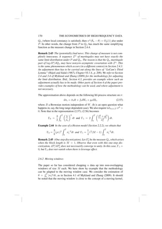
![METHODS BASED ON CONTIGUITY 171
and this may be a promising avenue of further investigation. See, in particular,
Linton (2007).
We use block length M, and equidistant times with spacing ∆tn = T/n. Also,
we use for simplicity
σ̃2
τn,i
=
1
∆tnMn
X
tn,j ∈(τn,i,τn,i+1]
(∆Xtn,j+1
)2
,
as estimator of σ2
τn,i
. The moving window estimate of θ is now
θ̃MW
n = (∆t)
n−M
X
i=0
^
|σtn,i
|r.
It is easy to see that
θ̃MW
n =
1
M
M
X
m=1
θ̃n,m + Op(n−1
),
where θ̃n,m is the non-overlapping block estimator, with block number one
starting at tn,m. In view of this representation, it is once again clear from suf-
ficiency considerations that the moving window estimator will have an asymp-
totic variance which is smaller (or, at least, no larger) than the estimator based
on non-overlapping blocks. We now carry out the precise asymptotic analysis.
To analyze this estimator, let M M, and let
An = {i = 0, ..., n − M : [tn,i, tn,i+M ] ⊆ [kM, (k + 1)M] for some k},
with Bn = {0, ..., n − M} − An. Write
n1/2
(θ̃MW
n − θ)
= n1/2
∆t
X
k
X
i:[tn,i,tn,i+M ]⊆[kM/n,(k+1)M/n]
( ^
|σtn,i
|r − |σtkM
|r
)
+ n1/2
∆t
X
i∈Bn
( ^
|σtn,i
|r − |σtn,i
|r
) + Op(n−1/2
). (2.58)
Now apply our methodology from Section 2.6.1, with block size M, to the
first term in (2.58). Under this block approximation, the inner sum in the first
term is based on conditionally i.i.d. observations, in fact, for [tn,i, tn,i+M ] ⊆
[kM/n, (k + 1)M/n], σ̃2
tn,i
= σ2
kM/nSi, in law, where
Si = M−1
i+M−1
X
j=i
U2
j , U0, U1, U2, ... iid standard normal. (2.59)
As in Section 4.1 of Mykland and Zhang (2009), there is no adjustment (à](https://image.slidesharecdn.com/i-241105032402-0ece1b19/85/I-A-1-Econometrics_of_High_Frequency_Data-pdf-63-320.jpg)
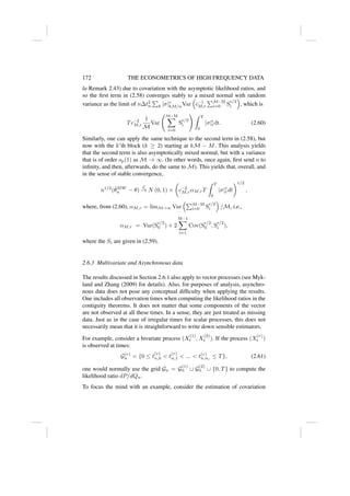
![METHODS BASED ON CONTIGUITY 173
under asynchronous data. It is shown in Mykland (2010a) that the Hayashi-
Yoshida estimator (Hayashi and Yoshida (2005)) can be seen as a nonpara-
metric maximum likelihood estimator (MLE). We shall here see that blocking
induces an additional class of local likelihood based MLEs. The difference be-
tween the former and the latter depends on the continuity assumptions made
on the volatility process, and is a little like the difference between the Kaplan-
Meier (Kaplan and Meier (1958)) and Nelson-Aalen (Nelson (1969), Aalen
(1976, 1978)) estimators in survival analysis. (Note that the variance estimate
for the Haysahi-Yoshida estimator from Section 5.3 of Mykland (2010a) obvi-
ously also remains valid in the setting of this paper).
For simplicity, work with a bivariate process, and let the grid Gn be given
by (2.61). For now, let the block dividers τ be any subset of Gn. Under the
approximate measure Qn, note that for
τn,i−1 ≤ t
(1)
n,j−1 t
(1)
n,j ≤ τn,i and τn,i−1 ≤ t
(2)
k−1 t
(2)
k ≤ τn,i (2.62)
the set of returns X
(1)
t
(1)
n,j
− X
(1)
t
(1)
n,j−1
and X
(2)
t
(2)
n,k
− X
(2)
t
(2)
n,k−1
are conditionally jointly
normal with mean zero and covariances
CovQn
((X
(r)
t
(r)
n,j
− X
(r)
t
(r)
n,j−1
, X
(s)
t
(s)
n,k
− X
(s)
t
(s)
n,k−1
) | Fτn,i−1
)
= (ζτn,i−1
)r,sd{(t
(r)
n,j−1, t
(r)
n,j) ∩ (t
(s)
n,k−1, t
(s)
n,k)}
where d is length (Lebesgue measure). Set
κr,s;j,k = ζd{(t
(r)
n,j−1, t
(r)
n,j) ∩ (t
(s)
n,k−1, t
(s)
n,k)}.
The Qn log likelihood ratio based on observations fully in block (τn,i−1, τn,i]
is therefore given as
`(ζ) = −
1
2
ln det(κ)
−
1
2
X
r,s,j,k
κr,s;j,k
(X
(r)
t
(r)
n,j
− X
(r)
t
(r)
n,j−1
)(X
(s)
t
(s)
n,k
− X
(s)
t
(s)
n,k−1
)
−
Ni
2
ln(2π),
where κr,s;j,k
are the elements of the matrix inverse of (κr,s;j,k), and Ni is
a measure of block sample size. The sum in (j, k) is over all intersections
(t
(r)
n,j−1, t
(r)
n,j) ∩ (t
(s)
n,k−1, t
(s)
n,k) with positive length satisfying (2.62). Call the
number of such terms
m
(r,s)
n,i = # nonempty intersections (t
(r)
n,j−1, t
(r)
n,j) ∩ (t
(s)
n,k−1, t
(s)
n,k)
satisfying (2.62) .](https://image.slidesharecdn.com/i-241105032402-0ece1b19/85/I-A-1-Econometrics_of_High_Frequency_Data-pdf-65-320.jpg)
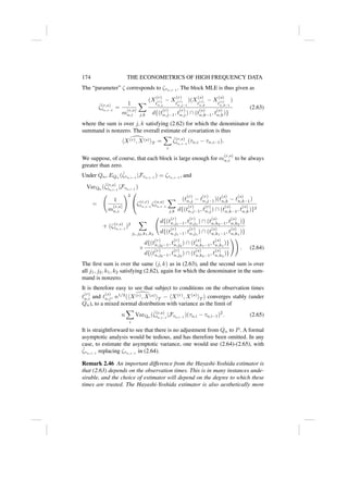
![METHODS BASED ON CONTIGUITY 175
pleasing. We note, however, that from likelihood considerations, the estima-
tor (2.63) will have an asymptotic variance which, as the block size tends to
infinity, converges to a limit which corresponds to the efficient minimum for
constant volatility matrix.
This phenomenon can be best illustrated for a scalar process (so there is no
asynchronicity). In this case, our estimator (2.63) of hX, XiT becomes (for
block size M fixed)
hX, XiT =
X
i
(τn,i − τn,i−1)
1
M
X
j: τn,i−1tn,j ≤τn,i
∆X2
tn,j
∆tn,j
. (2.66)
It is easy to see, by the methods in this paper, or directly, that for this esti-
mator, the asymptotic variance is 2T
R T
0 σ4
t dt, while for the standard realized
volatility, the corresponding expression is 2T
R T
0 σ4
t H0
(t)dt, where H(t) is
the asymptotic quadratic variation of time (2.39). It is always the case that
H0
(t) ≥ 1, and when observations are sufficiently irregular (under, say, Pois-
son sampling), the inequality is strict, cf. Section 2.7.2 below. Thus, (2.66) is
more efficient than regular realized volatility, but since the times can in many
cases not be trusted, the realized volatility remains a main tool for estimating
volatility.
2.6.4 More complicated data generating mechanisms
Jumps
We only consider the case of finitely many jumps (compound Poisson pro-
cesses, and similar). The conceptually simplest approach is to remove these
jumps using the kind of procedure described in Mancini (2001) and Lee and
Mykland (2006). The procedure will detect all intervals (tn,j−1, tn,j], with
probability tending to one (exponentially fast) as n → ∞. If one simply re-
moves the detected intervals from the analysis, it is easy to see that our asymp-
totic results go through unchanged.
The case of infinitely many jumps is more complicated, and beyond the scope
of this paper.
Note that there is a range of approaches for estimating the continuous part
of volatility in such data. Methods include bi- and multi-power (Barndorff-
Nielsen and Shephard (2004b)). Other devices are considered by Aı̈t-Sahalia
(2004), and Aı̈t-Sahalia and Jacod (2007). One can use our method of analysis
for all of these approaches.](https://image.slidesharecdn.com/i-241105032402-0ece1b19/85/I-A-1-Econometrics_of_High_Frequency_Data-pdf-67-320.jpg)
![176 THE ECONOMETRICS OF HIGH FREQUENCY DATA
Microstructure noise
The presence of noise does not alter the analysis in any major way. Suppose
one observes
Ytn,j
= Xtn,j
+ n,j
where the n,j’s are independent of the (Xt) process. The latter still follows
(2.25). We take the σ-field Xn,n to be generated by {Xtn,j
, n,j, 0 ≤ j ≤ n}.
Suppose that P1 and P2 are two measures on Xn,n for which: (1) the variables
{n,j, 0 ≤ j ≤ n} are independent of {Xtn,j
, 0 ≤ j ≤ n}, and (2) the
variables {n,j, 0 ≤ j ≤ n} have the same distribution under P1 and P2.
Then, from standard results in measure theory,
dP2
dP1
(Xtn,j
, n,j), 0 ≤ j ≤ n
=
dP2
dP1
Xtn,j
, 0 ≤ j ≤ n
.
The results in our theorems are therefore unchanged in the case of microstruc-
ture noise (unless one also wants to change the probability distribution of the
noise). We note that this remains the case irrespective of the internal depen-
dence structure of the noise.
The key observation which leads to this easy extension is that it is not required
for our results to work that the observables Ytn,j
generate the σ-field Xn,n. It
is only required that the observables be measurable with respect to this σ-field.
The same principle was invoked in Section 2.6.3.
The extension does not, obviously, solve all problems relating to microstructure
noise, since this type of data generating mechanism is best treated with an
asymptotics where M → ∞ as n → ∞. This is currently under investigation.
For one approach, see Mykland and Zhang (2011).
2.7 Irregularly spaced data
2.7.1 A second block approximation.
The approximation in Section 2.6.1 reduces the problem (in each block) to a
case of independent (but not identically distributed) increments. Can we do
better than this, and go to iid observations? We here give a criterion for this to
be the case.
Consider yet another approximate probability measure Rn, under which X0 =
x0, and
for each i = 1, ..., Kn : ∆Xtj+1
= στn,i−1
(
∆τi
∆tj+1Mi
)1/2
∆W∗
tj+1
for tn,j+1 ∈ (τn,i−1, τn,i]. (2.67)](https://image.slidesharecdn.com/i-241105032402-0ece1b19/85/I-A-1-Econometrics_of_High_Frequency_Data-pdf-68-320.jpg)
![IRREGULARLY SPACED DATA 177
Formally, we define the approximation as follows.
Definition 2.47 Rn is defined as Qn in Definition 2.42, but with (2.67) replac-
ing (2.53).
The crucial fact will be that under Rn, the observables ∆Xtj+1
are condition-
ally iid N(0, ζτn,i−1
∆τi/Mi) for tn,j+1 ∈ (τn,i−1, τn,i].
So that the following can be used together with the results in Mykland and
Zhang (2009), we will in the following let the process X be multivariate, and
we make the following assumption
Condition 2.48 (Structure of the instantaneous volatility). We assume that the
matrix process σt is itself an Itô processes, and that if λ
(p)
t is the smallest
eigenvalue of σt, then inft λ
(p)
t 0 a.s.
The contiguity question is then addressed as follows. Let P∗
n be the measure
from Remark 2.45 (corresponding to block length M = 1). Recall that
log
dRn
dP
= log
dRn
dQn
+ log
dQn
dP∗
n
+ log
dP∗
n
dP
.
Define
Bn,j = ∆tn,j+1
∆τn,i
Mi
−1
− 1
!
.
Theorem 2.49 (Asymptotic relationship between P∗
n, Qn and Rn). Assume
the conditions of Theorem 4 in Mykland and Zhang (2009), and let Z
(1)
n and
M
(1)
n be as in that theorem (see (2.71) and (2.74) in Section 2.7.3). Assume
that the following limits exist:
Γ2 =
p
2
lim
n→∞
X
j
B2
n,j and Γ3 =
p
2
lim
n→∞
X
j
log(1 + Bn,j).
Set
Z(2)
n =
1
2
X
i
X
tn,j ∈(τn,i−1,τn,i]
∆XT
tn,j
((σσT
)
−1
τn,i−1
)∆Xtn,j
× ∆t−1
n,j+1 −
∆τn,i
Mi
−1
!
,
and let M
(2)
n be the end point of the martingale part of Z
(2)
n (see (2.72) and
(2.74) in Section 2.7.3 for the explicit formula). Then, as n → ∞, (M
(1)
n , M
(2)
n )
converges stably in law under P∗
to a normal distribution with mean zero and
diagonal variance matrix with diagonal elements Γ1 and Γ2. Also, under P∗
,
log
dRn
dQn
= M(2)
n + Γ3 + op(1).](https://image.slidesharecdn.com/i-241105032402-0ece1b19/85/I-A-1-Econometrics_of_High_Frequency_Data-pdf-69-320.jpg)
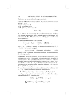
![IRREGULARLY SPACED DATA 179
since EU2
(1) = 2/(M + 1)(M + 2). Hence, both Γ2 and Γ3 are infinite. The
contiguity between Rn and the other probabilities fails. On the other hand all
our assumptions up to Section 2.6 are satisfied, and so P, P∗
n and Qn are all
contiguous. The AQVT (equation (2.39)) is given by H(t) = 2t . Also, if the
block size is constant (size M), the ADD is K(t) = (M − 1)t .
Example 2.52 (SYSTEMATIC IRREGULARITY.) Let be a small positive num-
ber, and let ∆tn,j = (1 + )T/n for odd j and ∆tn,j = (1 − )T/n for even
j (with ∆tn,n = T/n for odd n). Again, all our assumptions up to Section 2.6
are satisfied. The AQVT is given by H(t) = t(1 + 2
). If we suppose that all
Mi = 2, the ADD becomes K(t) = t. On the other hand, Bn,j = ±, so that,
again, both Γ2 and Γ3 are infinite. The contiguity between Rn and the other
probabilities thus fails in the same radical fashion as in the case of Poisson
sampling.
2.7.2 Irregular Spacing and Subsampling
We here return to a more direct study of the effect of irregular spacings. We
put ourselves in the situation from Section 2.4.3, where observation times are
independent of the process. As stated in equation (2.44), the limit law for the
realized volatility (for
√
n
[X, X]Gn
t − [X, X]t
) is mixed normal with (ran-
dom) variance
2T
Z t
0
σ4
s dHs,
where H is the asymptotic quadratic variation of time (AQVT). When obser-
vations are equidistant, H0
(t) ≡ 1. From the preceeding section, we also know
that if times are on the form (2.69), the asymptotic variance is unaffected. It is
worth elaborating on this in direct computation. Set
F(t) = lim
n→∞
1
n
#{tn,i+1 ≤ t}.
This quantity exists, if necessary by going through subsequences (Helly’s The-
orem, see, for example, p. 336 in Billingsley (1995)). Set
un,i = F(tn,i). (2.70)
Asymptotically, the un,i are equispaced:
1
n
#{un,i+1 ≤ t} =
1
n
#{tn,i+1 ≤ F(−1)
(t)} → F(F(−1)
(t)) = t
Inference is invariant to this transformation: Observing the process Xt at times
tn,i is the same as observing the process Yt = XF (−1)(t) at times un,i. If we
set U = {un,j, j = 0, ..., n}, then [X, X]G
T = [Y, Y ]U
T . Also, in the limit,](https://image.slidesharecdn.com/i-241105032402-0ece1b19/85/I-A-1-Econometrics_of_High_Frequency_Data-pdf-71-320.jpg)
![180 THE ECONOMETRICS OF HIGH FREQUENCY DATA
[X, X]T = [Y, Y ]T . Finally, the asymptotic distribution is the same in these
two cases.
If the un,i have AQVT U(t), the mixed normal variance transforms
2T
Z T
0
H0
(u)(hX, Xi0
t)2
dt = 2
Z 1
0
U0
(u)(hY, Y i0
t)2
dt.
The transformation (2.70) regularizes spacing. It means that without loss of
generality, one can take T = 1, F0
= 1 and U = H. Also, the transformation
(2.70) regularizes spacing defined by (2.69), and in this case, U0
(t) ≡ 1.
Example 2.53 On the other hand, it is clear from Example 2.51 that it is pos-
sible for U0
(t) to take other values than 1. The example shows that for Poisson
distributed observation times, H0
= U0
≡ 2, while, indeed F0
(t) ≡ 1/T.
The general situation can be expressed as follows:
Proposition 2.54 Assume that F exists and is monotonely increasing. Also
assume that H exists. Then U exists. For all s ≤ t, U(t) − U(s) ≥ t − s.
In particular, if U0
(t) exists, then U0
(t) ≥ 1. The following statements are
equivalent:
(i) U(1) = 1
(ii) U0
≡ 1
(iii)
Pn
j=0 un,j+1 − un,j − 1
n
2
= op(n−1
).
Proof of Proposition 2.54. The first statement uses a standard property of the
variance: if ∆tn,j+1 = tn,j+1 − tn,j, and ∆n = T/n, then
n
T
X
tn,j+1≤t
(∆tn,j+1)2
=
n
T
X
tn,j+1≤t
(∆tn,j+1 − ∆n)2
+
n
T
#{tn,i+1 ≤ t}(∆n)2
≥
n
T
#{tn,i+1 ≤ t}(∆n)2
.
By taking limits as n → ∞ under F0
(t) ≡ 1/T, we get that H(t) − H(s) ≥
t − s. In particular, the same will be true for U.
The equivalence between (i) and (iii) follows from the proof of Lemma 2 (p.
1029) in Zhang (2006). (The original lemma uses slightly different assump-
tions). 2
The implication of the proposition is that under the scenario U(1) = 1, ob-
servation times are “almost” equidistant. In particular, subsampling does not
change the structure of the spacings. On the other hand, when U(1) 1, there
is scope for subsampling to regularize the times.](https://image.slidesharecdn.com/i-241105032402-0ece1b19/85/I-A-1-Econometrics_of_High_Frequency_Data-pdf-72-320.jpg)
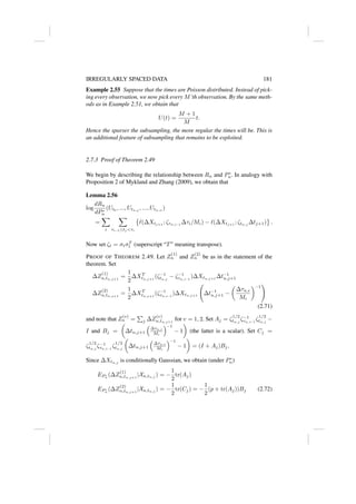


![[DSC Europe 25] Ivan Lukovic & Marija Djukic - From Data to Value: Why Maturi...](https://cdn.slidesharecdn.com/ss_thumbnails/ahrfps8xr6knowwhacxh-1-ivan-marija-dsc-2025-ld-v1-presentation-260115093812-be21adfc-thumbnail.jpg?width=640&height=640&fit=bounds)


![[DSC Europe 25] Andrzej Kowalczyk - AI - how to start small and grow in the f...](https://cdn.slidesharecdn.com/ss_thumbnails/oy1zmo94qv6vpcqjvno2-andrzej-kowalczyk-ai-how-to-start-small-and-grow-in-the-future-1-260119121559-cf093b23-thumbnail.jpg?width=640&height=640&fit=bounds)


