This document outlines key concepts related to long-term investment opportunities and frictions. It discusses how investment opportunities depend on state variables that influence returns and risks over time. It also introduces the concepts of equivalent safe rate and equivalent annuity, which define the optimal growth rate of wealth or utility for a long-term investor. The document proposes solving for long-term optimal portfolios using duality bounds, stationary equations, and criteria for long-run optimality.

![Long Run and Stochastic Investment Opportunities
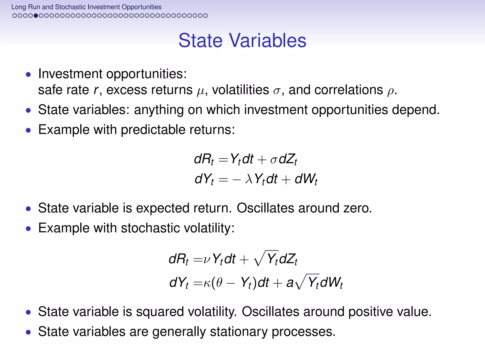
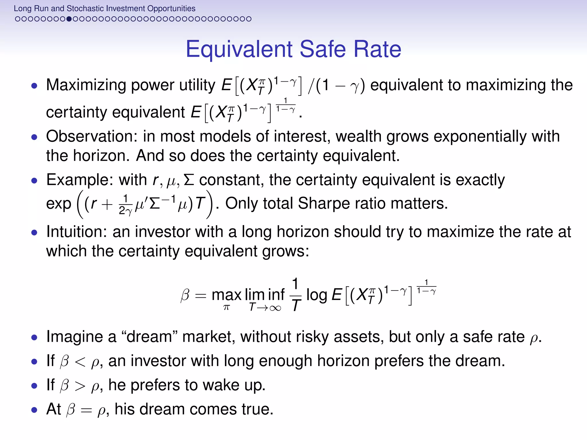
Utility Maximization
• Basic portfolio choice problem: maximize utility from terminal wealth:
π
max E[U(XT )]
π
• Easy for logarithmic utility U(x) = log x.
Myopic portfolio π = Σ−1 µ optimal. Numeraire argument.
• Portfolio does not depend on horizon (even random!), and on the
dynamics of the the state variable, but only its current value.
• But logarithmic utility leads to counterfactual predictions.
And implies that unhedgeable risk premia η are all zero.
• Power utility U(x) = x 1−γ /(1 − γ) is more flexible.
Portfolio no longer myopic. Risk premia η nonzero, and depend on γ.
• Power utility far less tractable.
Joint dependence on horizon and state variable dynamics.
• Explicit solutions few and cumbersome.
• Goal: keep dependence from state variable dynamics, lose from horizon.
• Tool: assume long horizon.](https://image.slidesharecdn.com/lisbonlectures-120708172712-phpapp01/75/UT-Austin-Portugal-Lectures-on-Portfolio-Choice-5-2048.jpg)

![Long Run and Stochastic Investment Opportunities
Duality Bound
π η
• For any payoff X = and any discount factor M = MT , E[XM] ≤ x.
XT
Because XM is a local martingale.
• Duality bound for power utility:
γ
1
1−γ
E X 1−γ 1−γ
≤ xE M 1−1/γ
• Proof: exercise with Hölder’s inequality.
• Duality bound for exponential utility:
1 x 1 M M
− log E e−αX ≤ + E log
α E[M] α E[M] E[M]
• Proof: Jensen inequality under risk-neutral densities.
• Both bounds true for any X and for any M.
Pass to sup over X and inf over M.
• Note how α disappears from the right-hand side.
• Both bounds in terms of certainty equivalents.
• As T → ∞, bounds for equivalent safe rate and annuity follow.](https://image.slidesharecdn.com/lisbonlectures-120708172712-phpapp01/75/UT-Austin-Portugal-Lectures-on-Portfolio-Choice-15-2048.jpg)


![Long Run and Stochastic Investment Opportunities
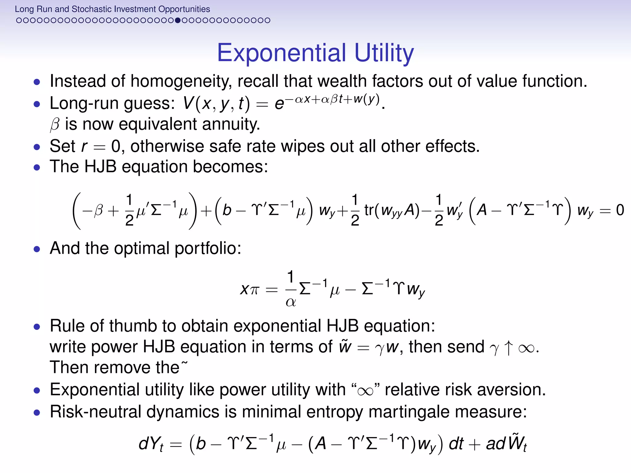
Exponential Utility
Theorem
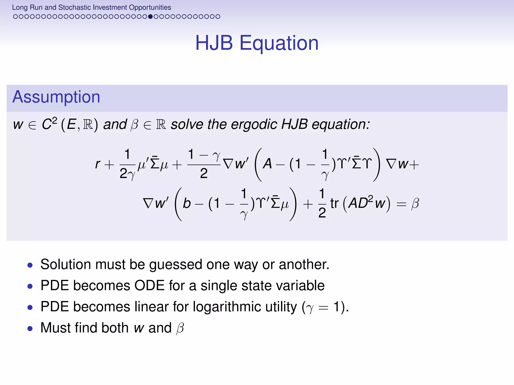
If r = 0 and w solves equation:
1 ¯ 1 ¯ ¯ 1
µ Σµ − w A − Υ ΣΥ w+ w b − Υ Σµ + tr AD 2 w = β
2 2 2
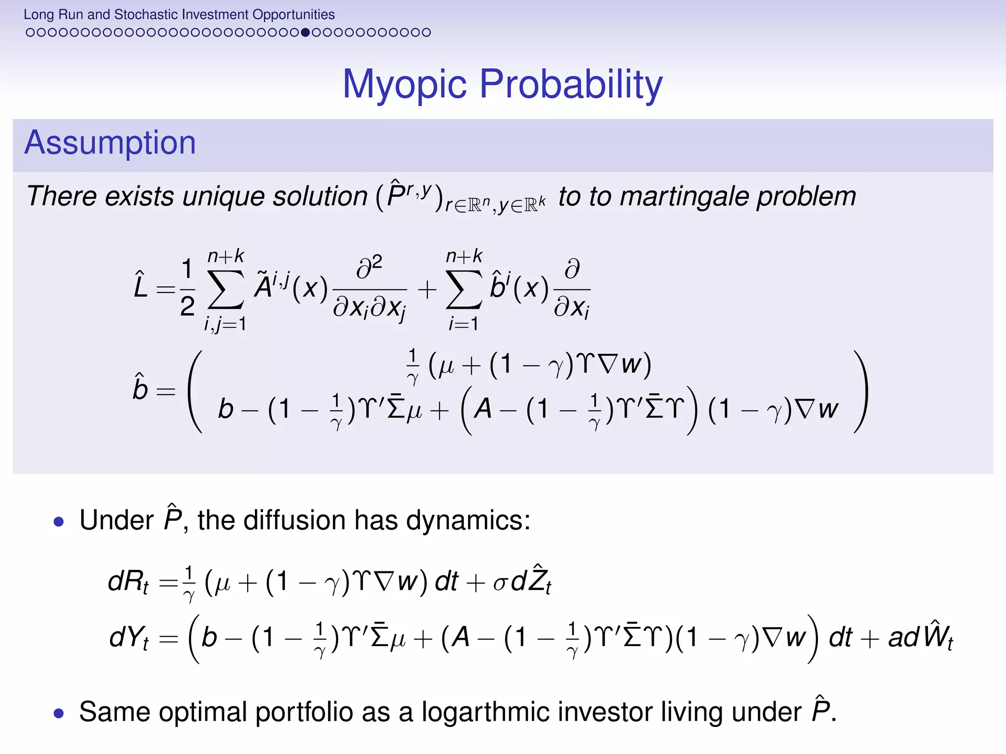
and myopic dynamics is well posed:
ˆ
dRt =σd Zt
¯ ¯ ˆ
dYt = b − Υ Σµ − (A − Υ ΣΥ) w dt + ad Wt
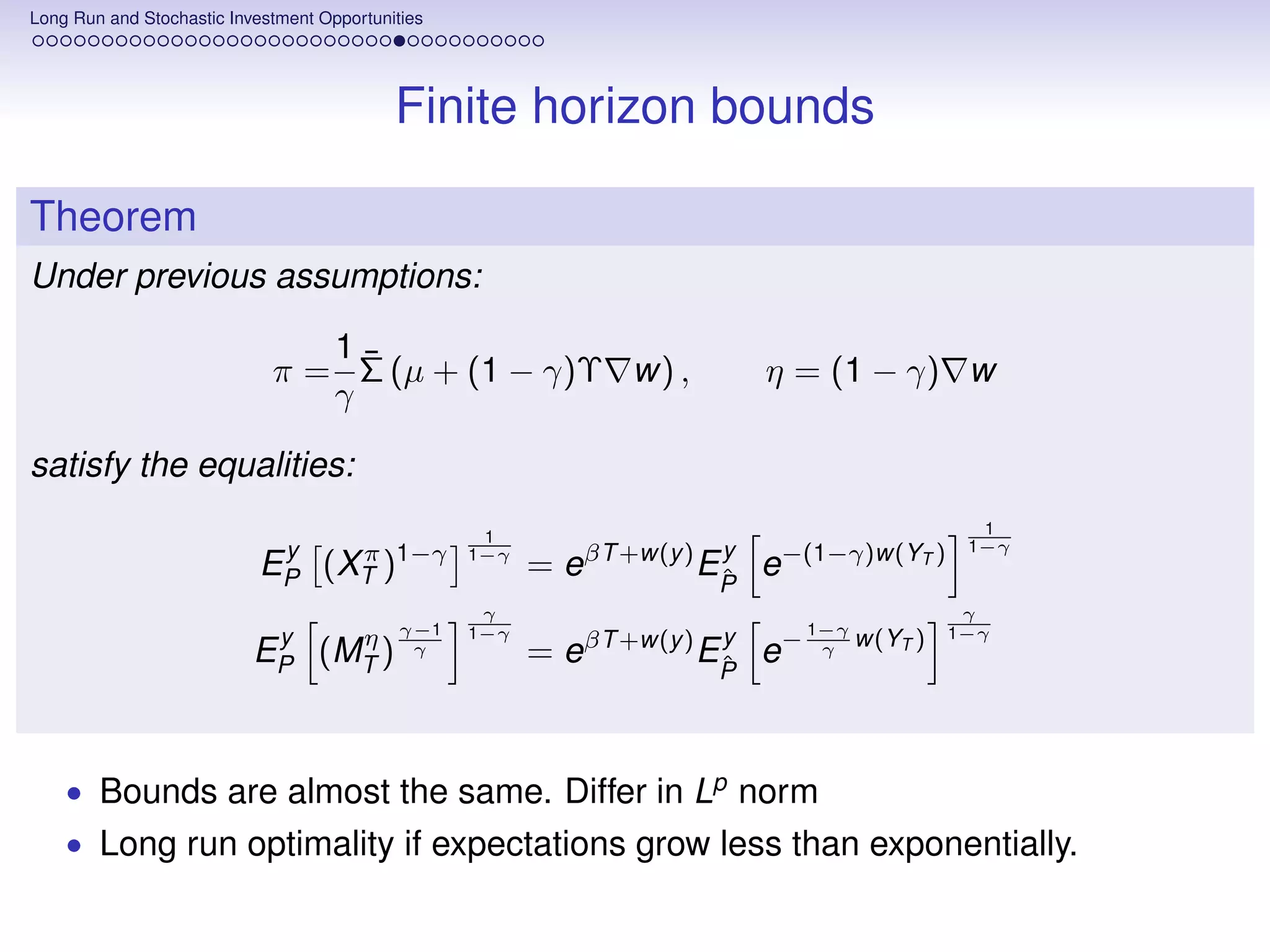
Then for the portfolio and risk premia (π, η) given by:
1
xπ = Σ−1 µ − Σ−1 Υ w η=− w
α
finite-horizon bounds hold as:
1 y π 1 y
− log EP e−α(XT −x) =βT + log EP ew(y )−w(YT )
ˆ
α α
1 y η 1 y
EP [M log M η ] =βT + EP [w(y ) − w(YT )]
2 α ˆ](https://image.slidesharecdn.com/lisbonlectures-120708172712-phpapp01/75/UT-Austin-Portugal-Lectures-on-Portfolio-Choice-36-2048.jpg)
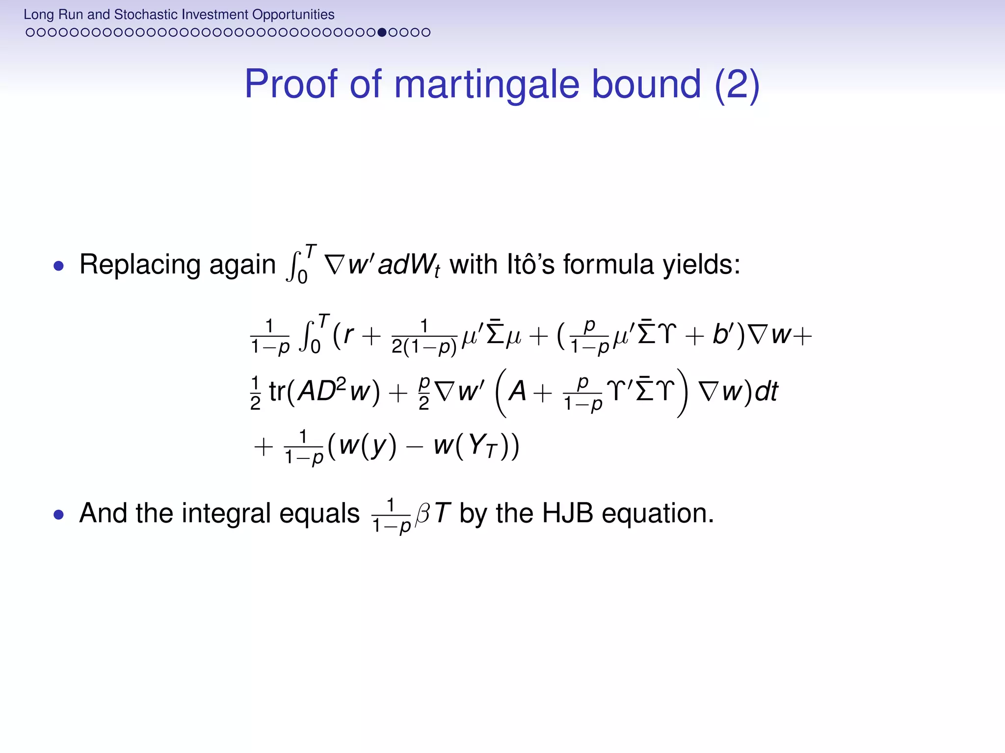
![Long Run and Stochastic Investment Opportunities
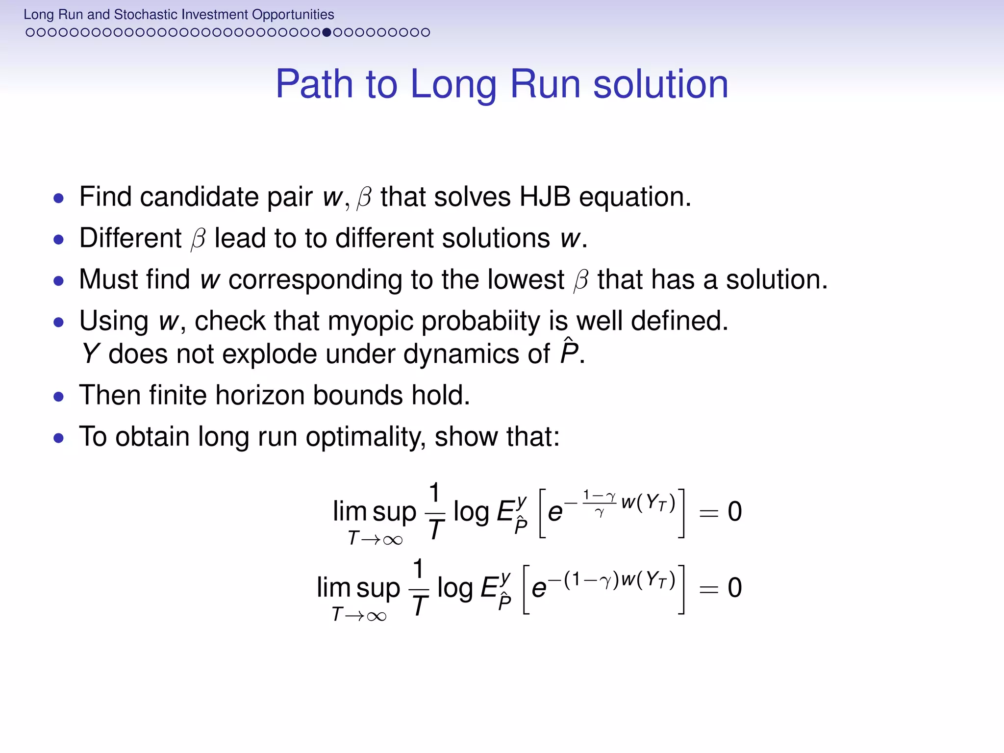
Proof of Long-Run Optimality (1)
• By the duality bound:
1 1 y η 1 1−p y
0 ≤ lim inf log EP (MT )q log EP [(XT )p ]
− π
T →∞ p T T
1 y η 1−p 1 y
≤ lim sup log EP (MT )q − lim inf log EP [(XT )p ]
π
T →∞ pT T →∞ pT
1−p y 1 1 y
= lim sup log EP e− 1−p v (YT ) − lim inf
ˆ log EP e−v (YT )
ˆ
T →∞ pT T →∞ pT
• For p < 0 enough to show lower bound
1 y 1
lim inf log EP exp − 1−p v (YT )
ˆ ≥0
T →∞ T
and upper bound:
1 y
lim supT →∞ T log EP [exp (−v (YT ))] ≤ 0
ˆ
• Lower bound follows from tightness.](https://image.slidesharecdn.com/lisbonlectures-120708172712-phpapp01/75/UT-Austin-Portugal-Lectures-on-Portfolio-Choice-38-2048.jpg)

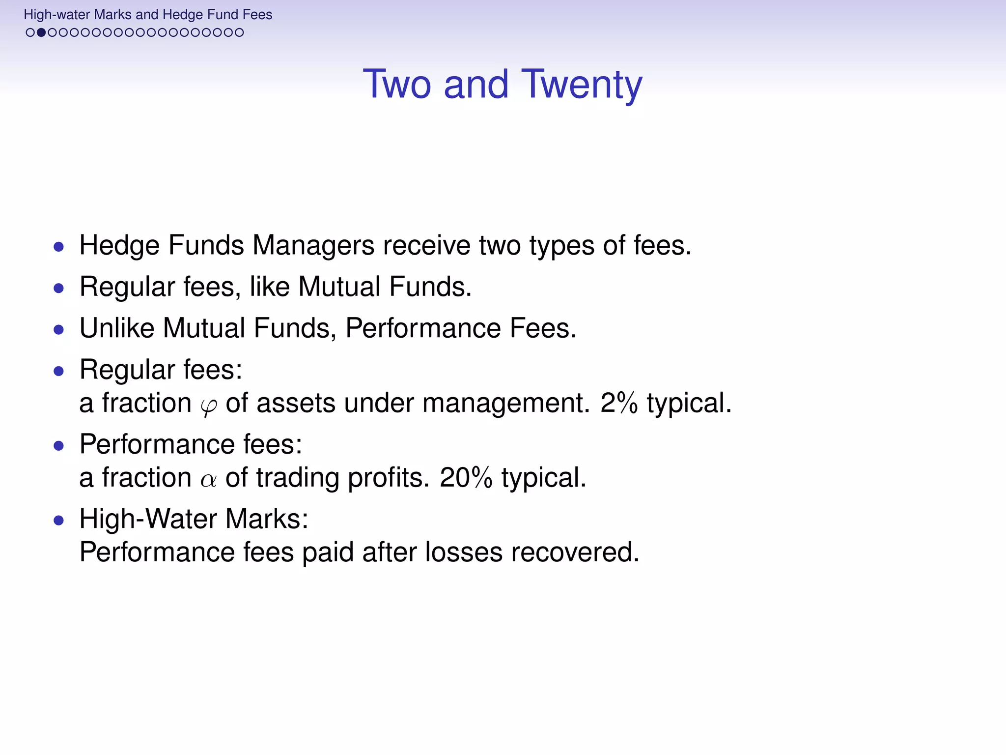


![High-water Marks and Hedge Fund Fees
Long Horizon
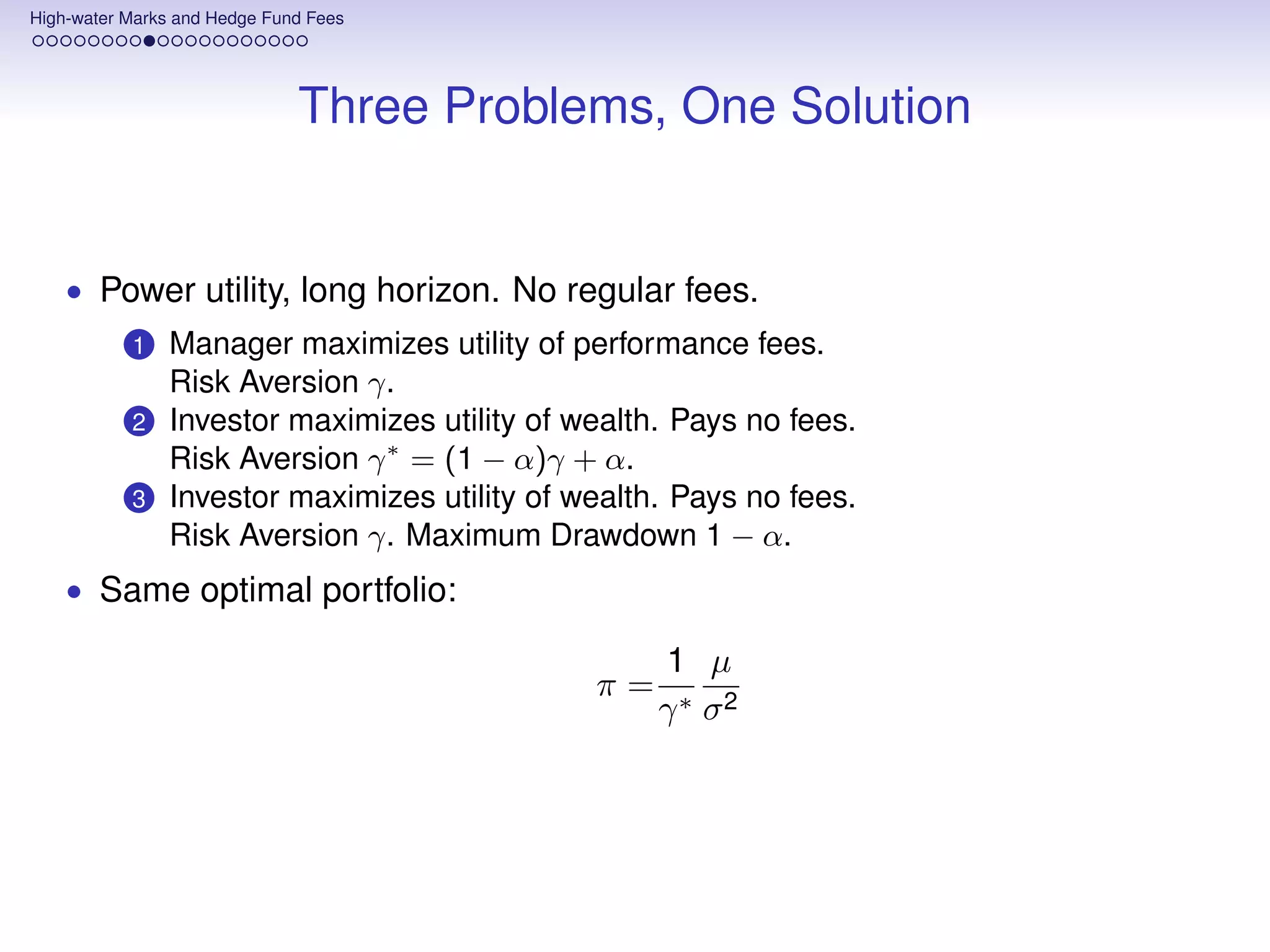
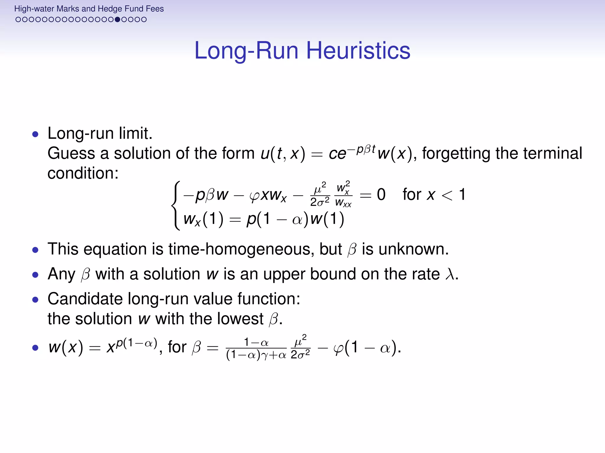
• The manager chooses the portfolio π which maximizes expected power
utility from fees at a long horizon.
• Maximizes the long-run objective:
1 p
max lim log E[FT ] = β
π T →∞ pT
• Dumas and Luciano (1991), Grossman and Vila (1992), Grossman and
Zhou (1993), Cvitanic and Karatzas (1995). Risk-Sensitive Control:
Bielecki and Pliska (1999) and many others.
2
1 µ
• β=r+ γ 2σ 2 for Merton problem with risk-aversion γ = 1 − p.](https://image.slidesharecdn.com/lisbonlectures-120708172712-phpapp01/75/UT-Austin-Portugal-Lectures-on-Portfolio-Choice-52-2048.jpg)
![High-water Marks and Hedge Fund Fees
Solving It
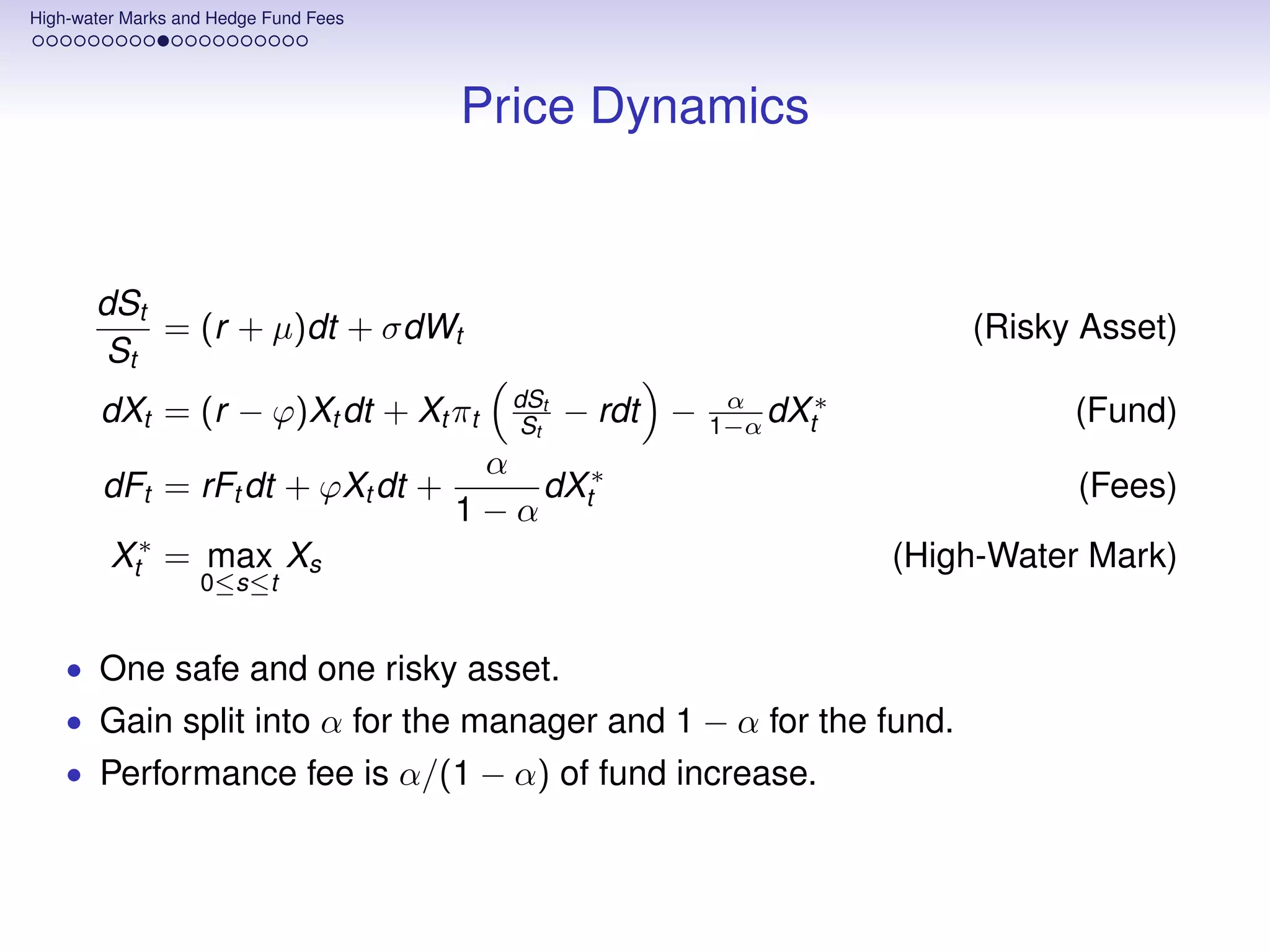
• Set r = 0 and ϕ = 0 to simplify notation.
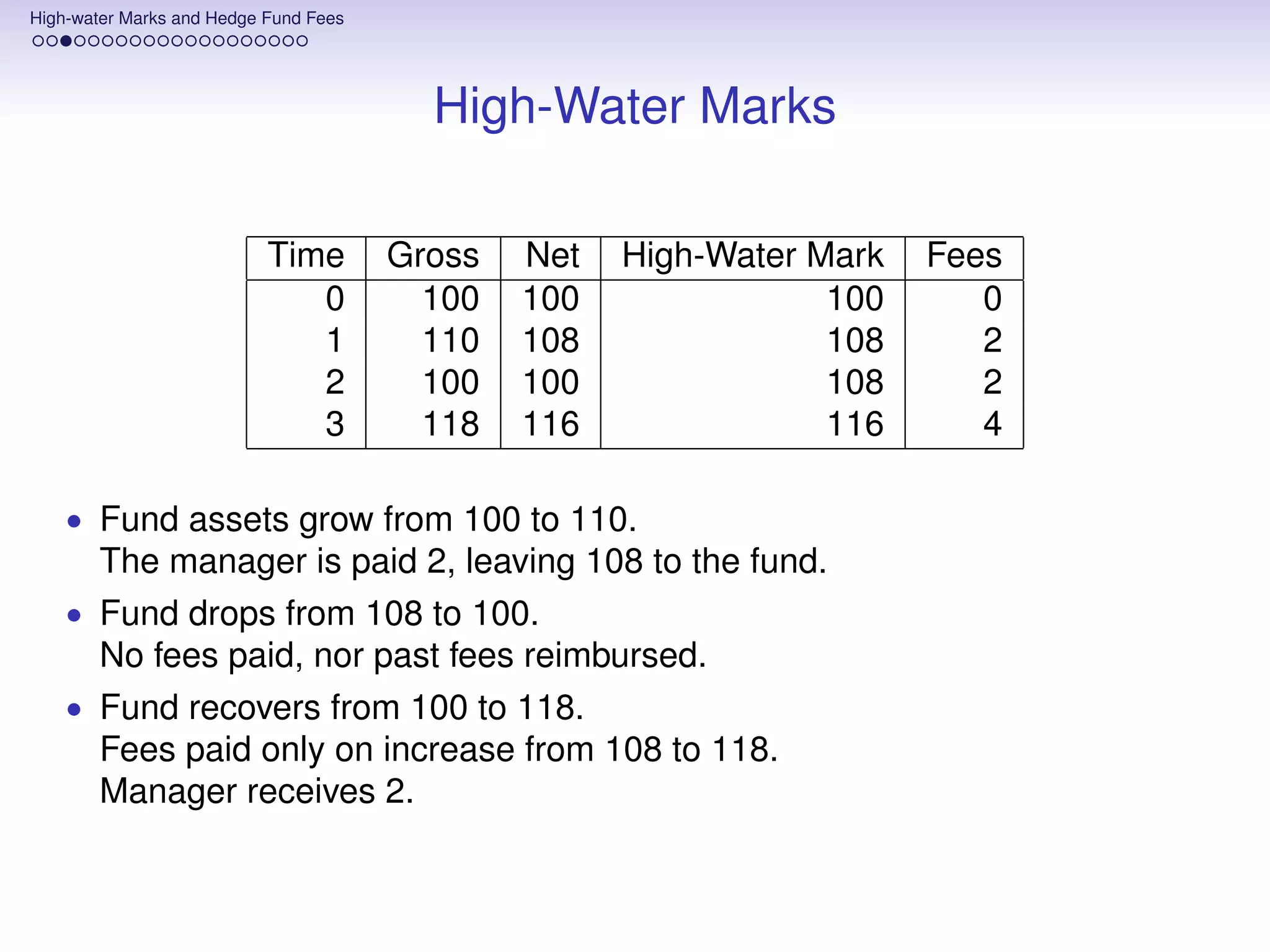
• Cumulative fees are a fraction of the increase in the fund:
α
Ft = (X ∗ − X0 )
∗
1−α t
• Thus, the manager’s objective is equivalent to:
1 ∗
max lim log E[(XT )p ]
π T →∞ pT
• Finite-horizon value function:
1
V (x, z, t) = sup E[XT p |Xt = x, Xt∗ = z]
∗
π p
1
dV (Xt , Xt∗ , t) = Vt dt + Vx dXt + Vxx d X t + Vz dXt∗
2
2
= Vt dt + Vz − α
1−α Vx dXt∗ + Vx Xt (πt µ − ϕ)dt + Vxx σ πt2 Xt2 dt
2](https://image.slidesharecdn.com/lisbonlectures-120708172712-phpapp01/75/UT-Austin-Portugal-Lectures-on-Portfolio-Choice-53-2048.jpg)

![High-water Marks and Hedge Fund Fees
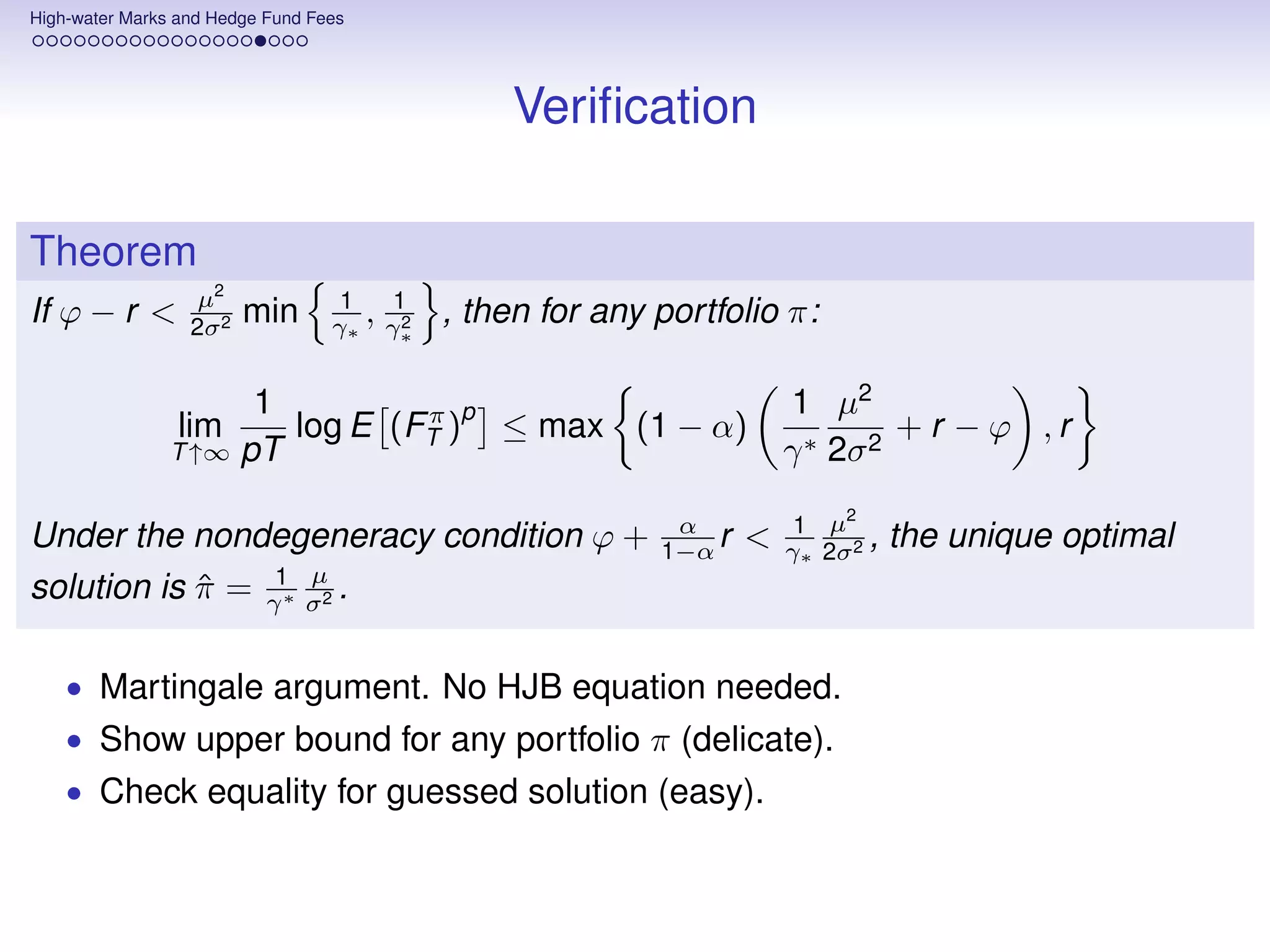
Upper Bound (1)
• Take p > 0 (p < 0 symmetric).
• For any portfolio π:
T σ2 2 T ˜
RT = − π dt
0 2 t
+ 0
σπt d Wt
˜
• Wt = Wt + µ/σt risk-neutral Brownian Motion
• Explicit representation:
∗ ∗ µ ˜ µ2
E[(XT )p ] = E[ep(1−α)RT ] = EQ ep(1−α)RT e σ WT − 2σ2 T
π
• For δ > 1, Hölder’s inequality:
δ−1
δ µ ˜ µ2 δ
µ2
σ WT − 2σ 2
µ ˜ 1 T
∗ ∗
σ WT − 2σ 2 T
p(1−α)RT δp(1−α)RT δ δ−1
EQ e e ≤ EQ e EQ e
1 µ2
• Second term exponential normal moment. Just e δ−1 2σ2 T .](https://image.slidesharecdn.com/lisbonlectures-120708172712-phpapp01/75/UT-Austin-Portugal-Lectures-on-Portfolio-Choice-57-2048.jpg)
![High-water Marks and Hedge Fund Fees
Upper Bound (2)
∗
• Estimate EQ eδp(1−α)RT .
• Mt = eRt strictly positive continuous local martingale.
Converges to zero as t ↑ ∞.
• Fact:
inverse of lifetime supremum (M∞ )−1 uniform on [0, 1].
∗
• Thus, for δp(1 − α) < 1:
∗ ∗ 1
EQ eδp(1−α)RT ≤ EQ eδp(1−α)R∞ =
1 − δp(1 − α)
• In summary, for 1 < δ < 1
p(1−α) :
1 π p 1 µ2
lim log E (FT ) ≤
T ↑∞ pT p(δ − 1) 2σ 2
• Thesis follows as δ → 1
p(1−α) .](https://image.slidesharecdn.com/lisbonlectures-120708172712-phpapp01/75/UT-Austin-Portugal-Lectures-on-Portfolio-Choice-58-2048.jpg)

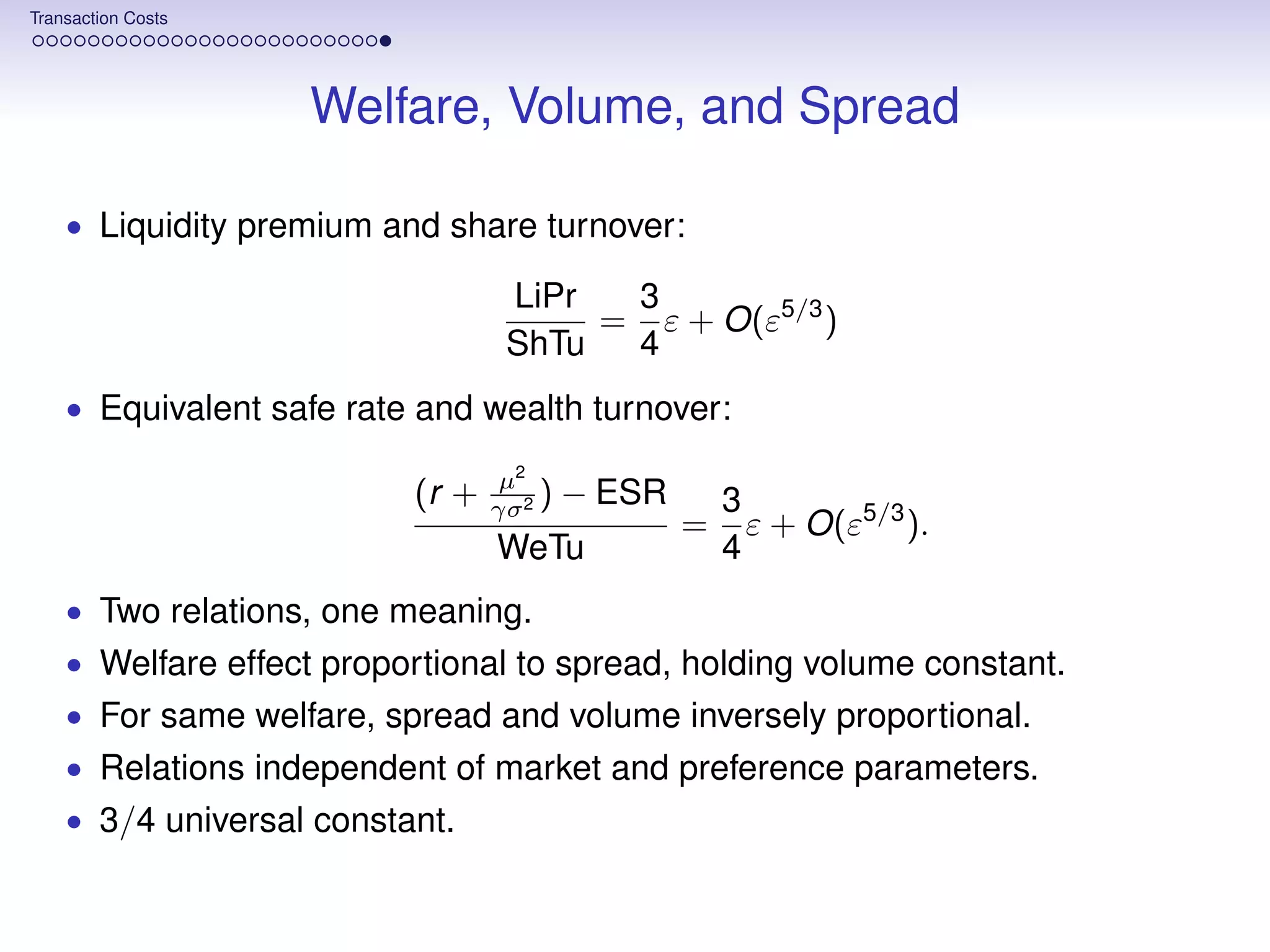
![Transaction Costs
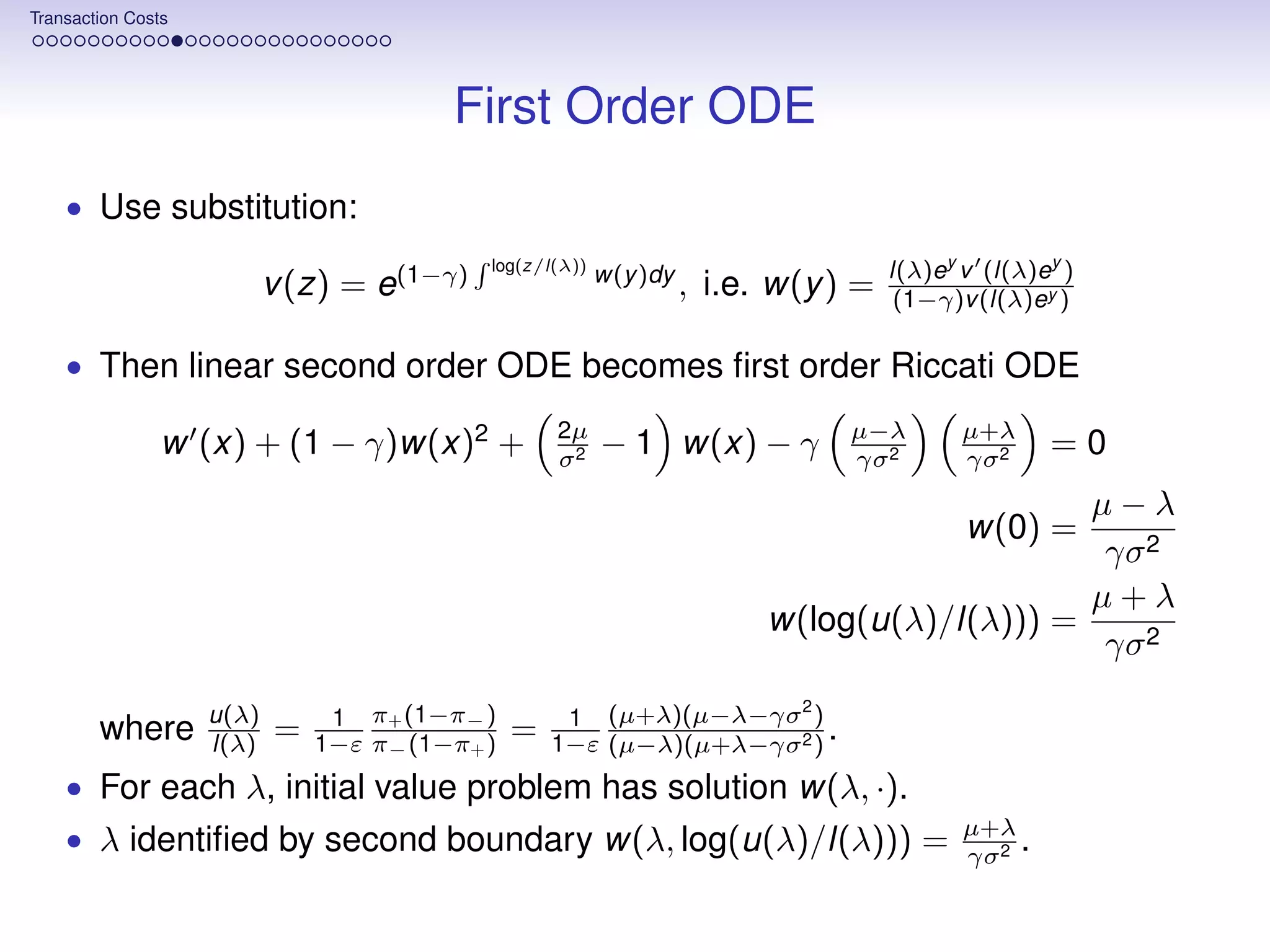
Explicit Solutions
• First, solve ODE for w(x, λ). Solution (for positive discriminant):
a(λ) tan[tan−1 ( b(λ) ) + a(λ)x] + ( σ2 − 2 )
a(λ)
µ 1
w(λ, x) = ,
γ−1
where
2 2
2
−λ
a(λ) = (γ − 1) µγσ4 − 1
2 − µ
σ2
, b(λ) = 1
2 − µ
σ2
+ (γ − 1) µ−λ .
γσ 2
• Similar expressions for zero and negaive discriminants.](https://image.slidesharecdn.com/lisbonlectures-120708172712-phpapp01/75/UT-Austin-Portugal-Lectures-on-Portfolio-Choice-71-2048.jpg)
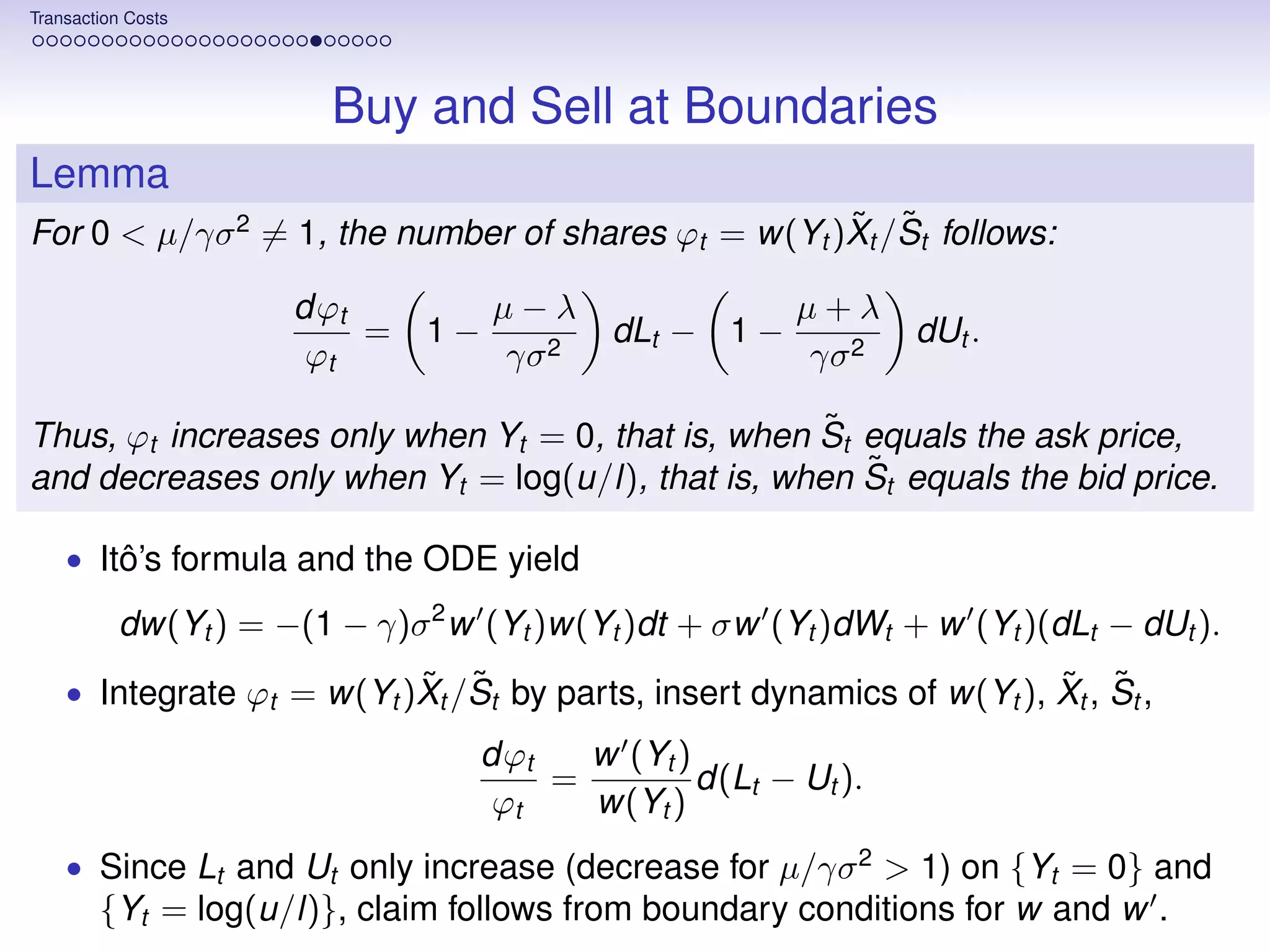
![Transaction Costs
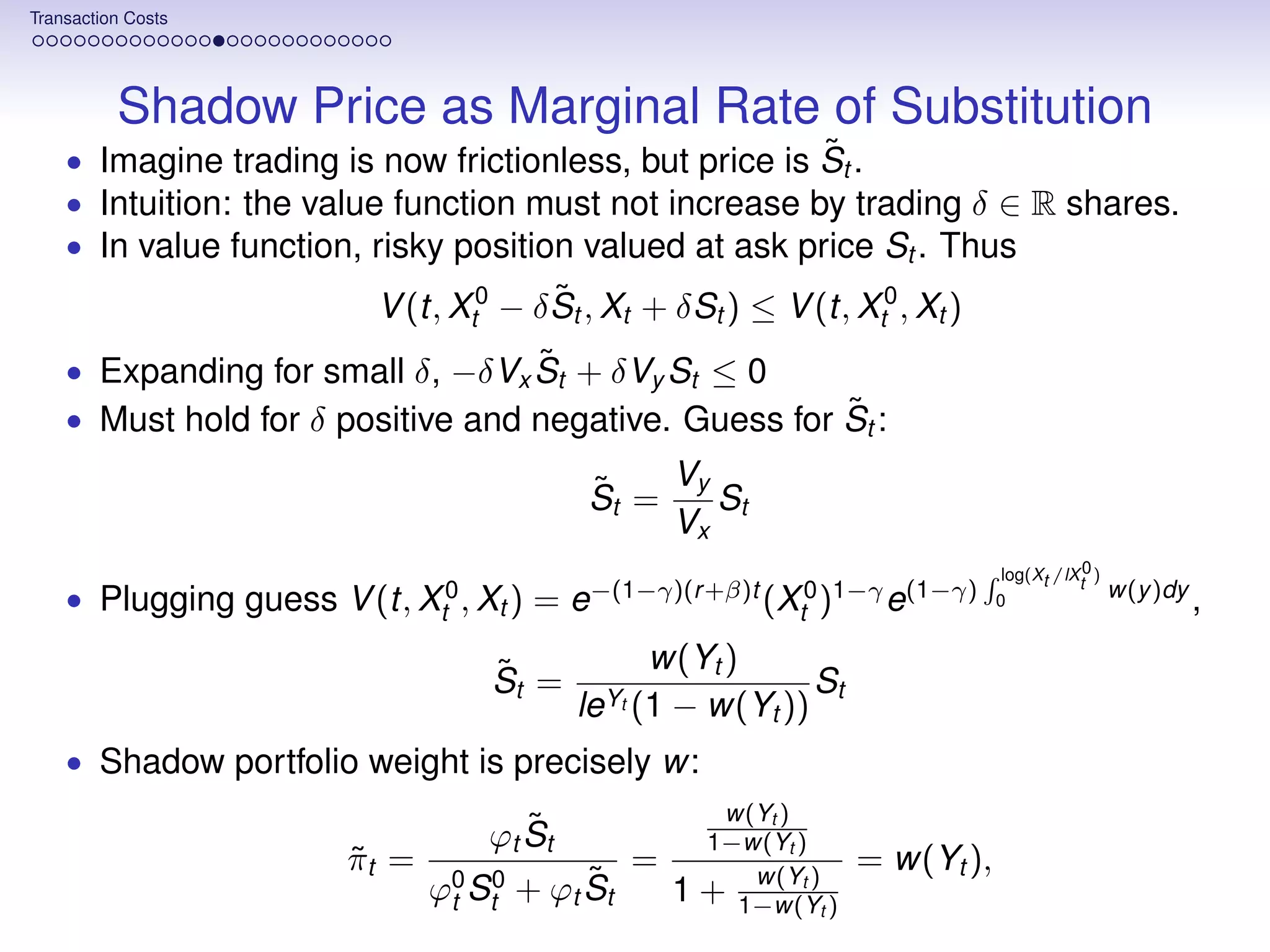
Construction of Shadow Price
• So far, a string of guesses. Now construction.
• Define Yt as reflected diffusion on [0, log(u/l)]:
dYt = (µ − σ 2 /2)dt + σdWt + dLt − dUt , Y0 ∈ [0, log(u/l)],
Lemma
˜ w(Y )
The dynamics of S = S leY (1−w(Y )) is given by
˜ ˜
d S(Yt )/S(Yt ) = (˜(Yt ) + r ) dt + σ (Yt )dWt ,
µ ˜
where µ(·) and σ (·) are defined as
˜ ˜
σ 2 w (y ) w (y ) σw (y )
µ(y ) =
˜ − (1 − γ)w(y ) , σ (y ) =
˜ .
w(y )(1 − w(y )) 1 − w(y ) w(y )(1 − w(y ))
˜
And the process S takes values within the bid-ask spread [(1 − ε)S, S].](https://image.slidesharecdn.com/lisbonlectures-120708172712-phpapp01/75/UT-Austin-Portugal-Lectures-on-Portfolio-Choice-75-2048.jpg)
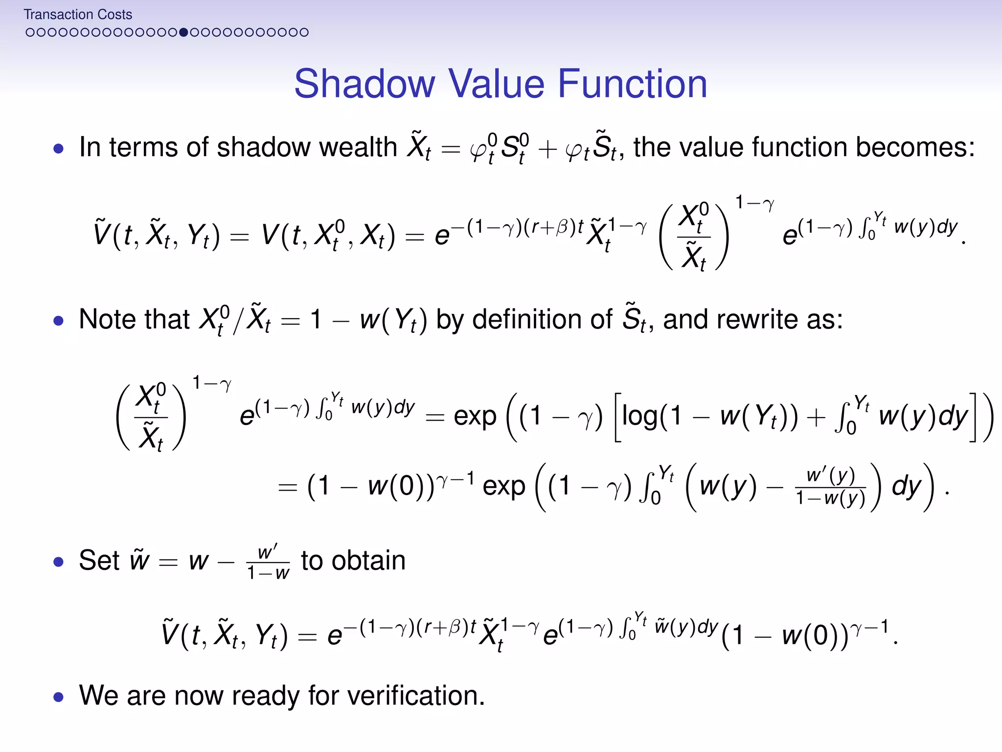
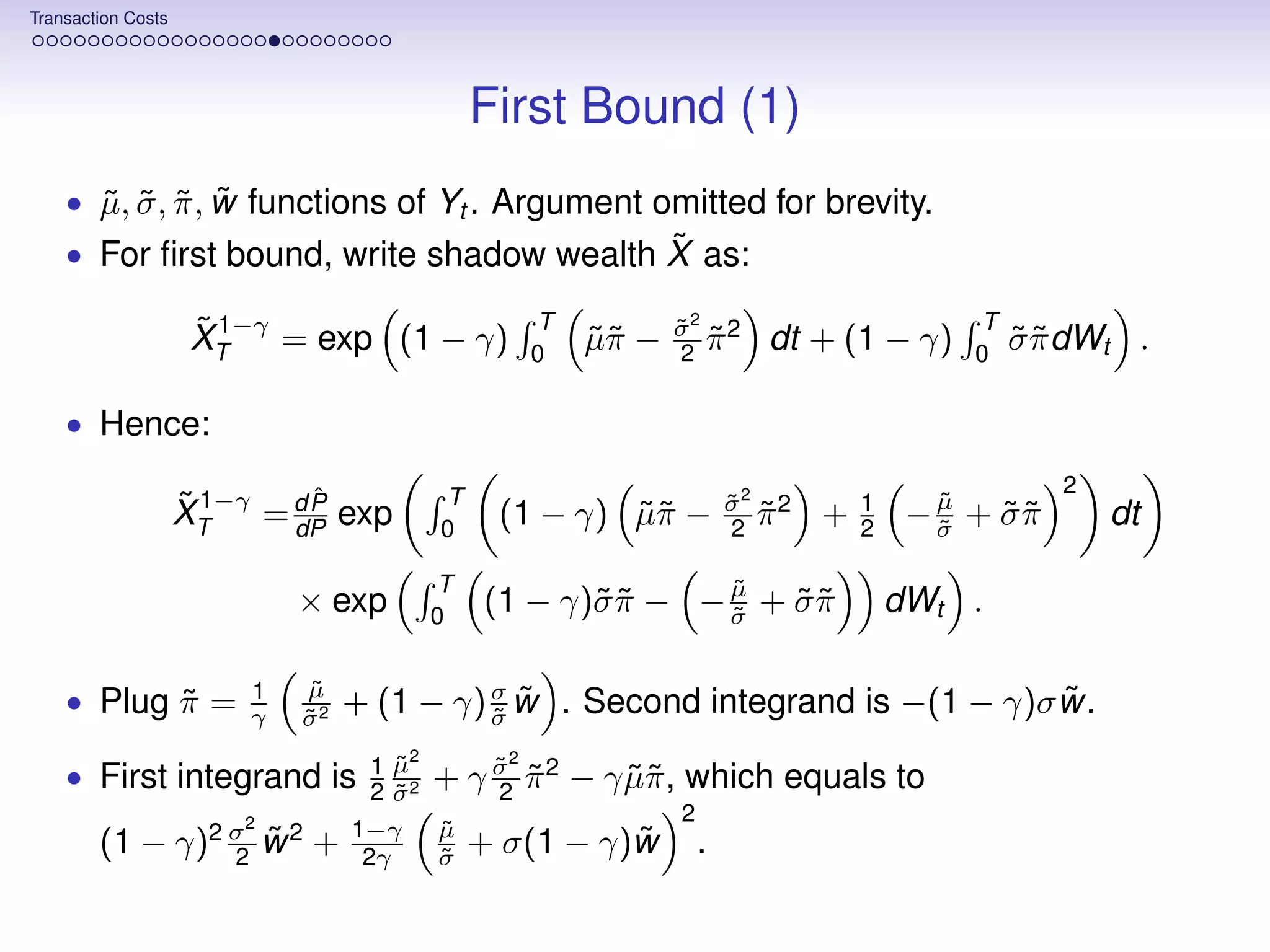
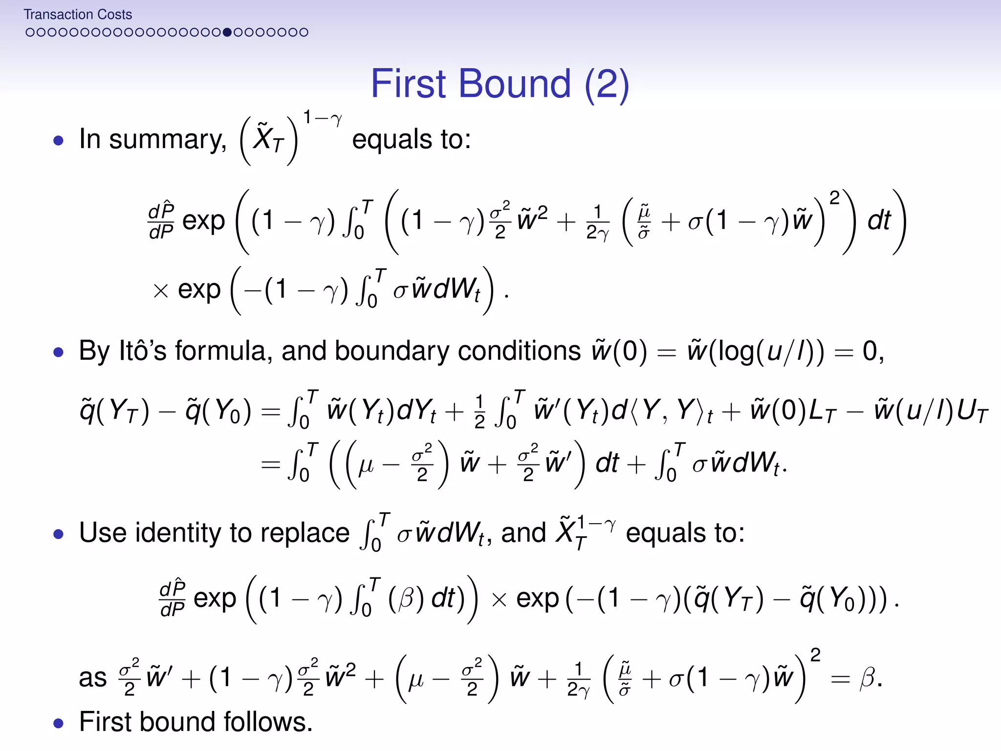
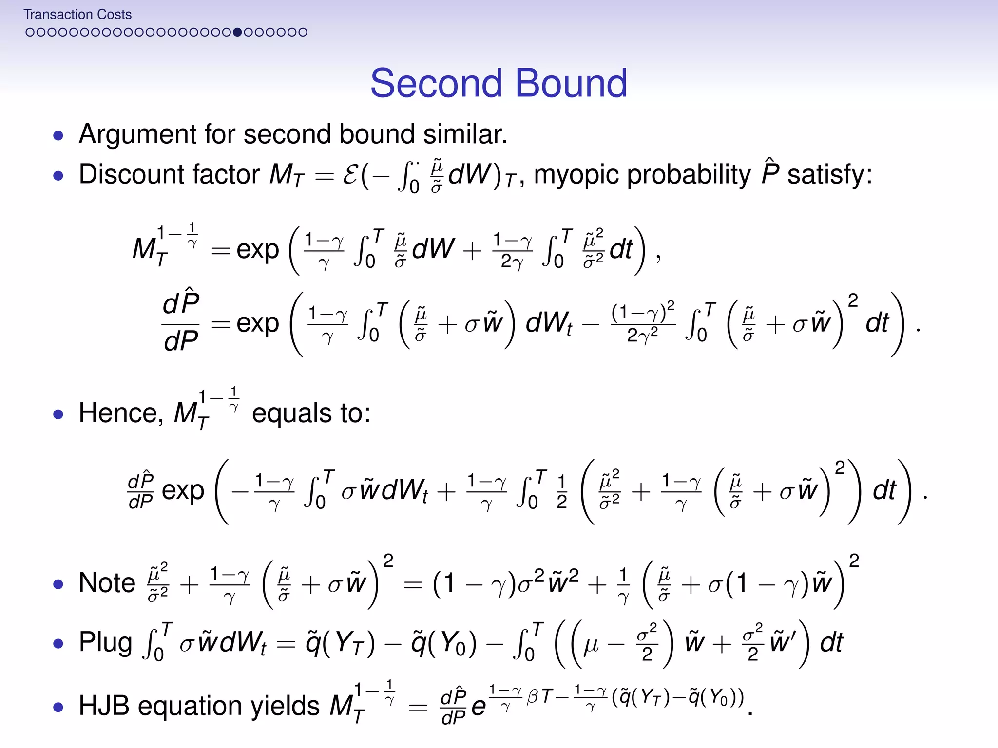
![Transaction Costs
Finite-horizon Bound
Theorem
˜
The shadow payoff XT of the portfolio π = w(Yt ) and the shadow discount
˜
· µ
˜ y
˜
factor MT = E(− 0 σ dWt )T satisfy (with q (y ) =
˜
˜
w(z)dz):
˜ 1−γ =e(1−γ)βT E e(1−γ)(q (Y0 )−q (YT )) ,
E XT ˆ ˜ ˜
1
γ γ
1− γ 1 ˜ ˜
E MT =e(1−γ)βT E e( γ −1)(q (Y0 )−q (YT ))
ˆ .
ˆ ˆ
where E[·] is the expectation with respect to the myopic probability P:
ˆ T T 2
dP µ
˜ 1 µ
˜
= exp − + σ π dWt −
˜˜ − + σπ
˜˜ dt .
dP 0 σ
˜ 2 0 σ
˜](https://image.slidesharecdn.com/lisbonlectures-120708172712-phpapp01/75/UT-Austin-Portugal-Lectures-on-Portfolio-Choice-76-2048.jpg)
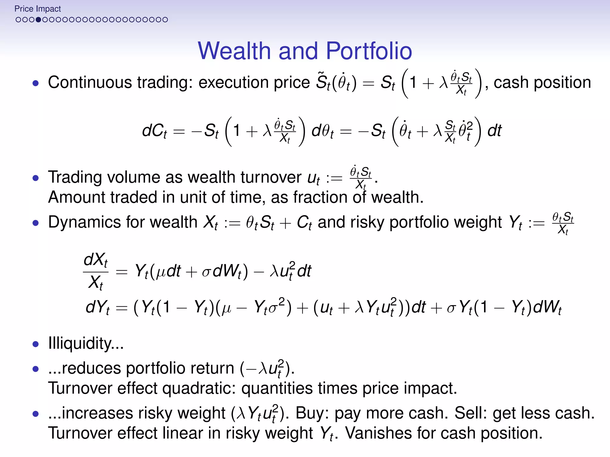
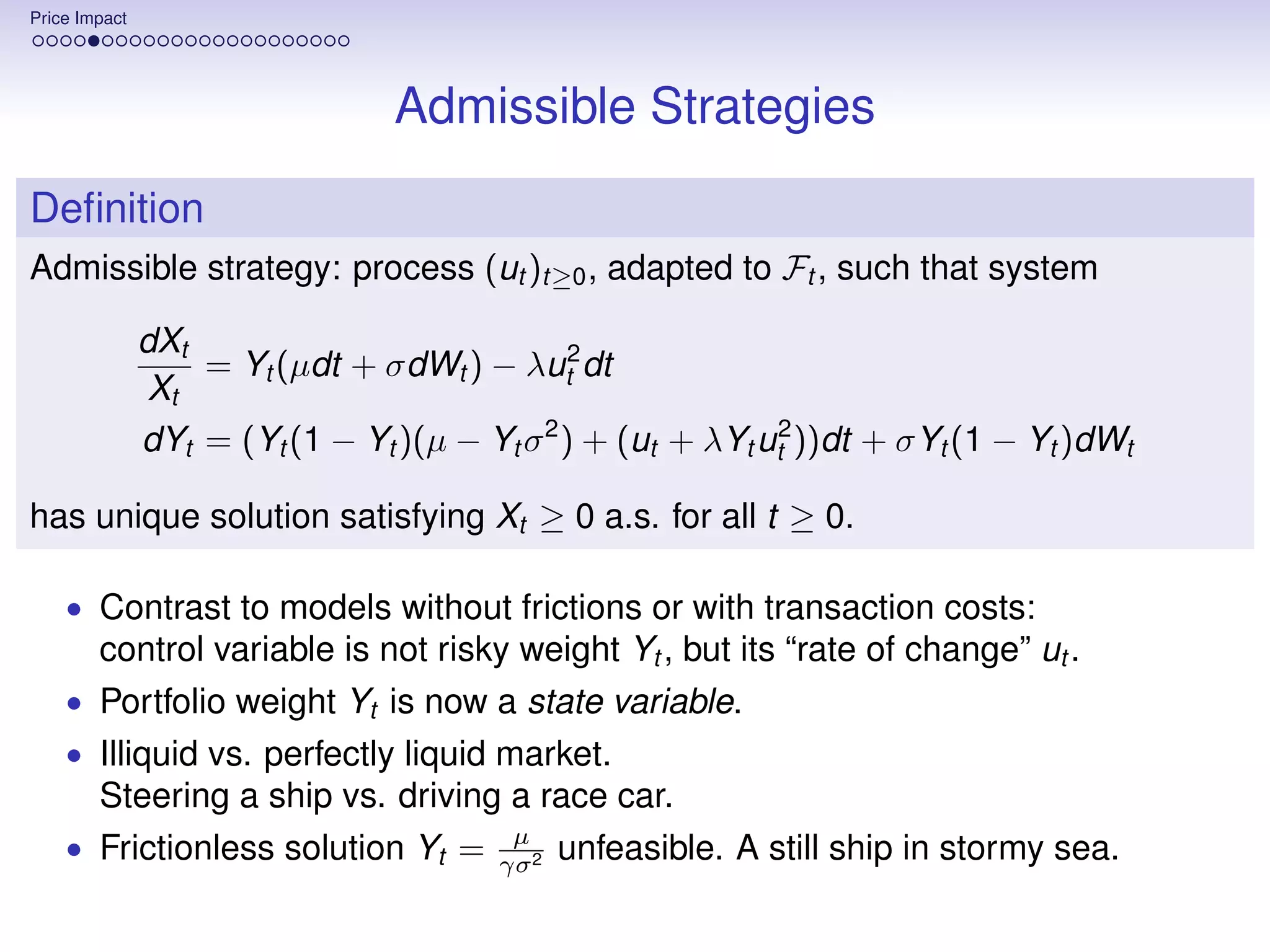
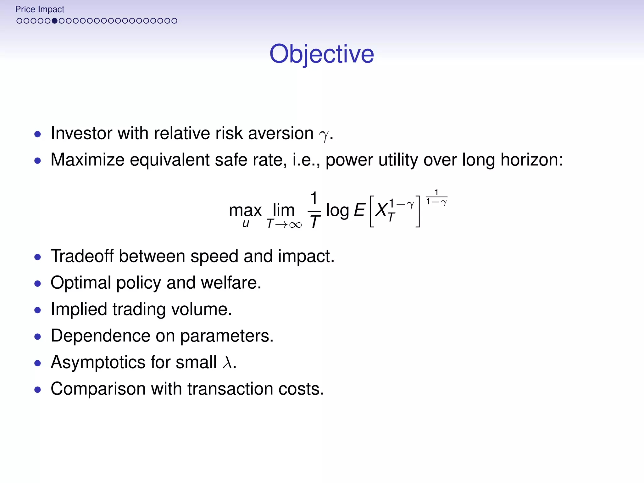
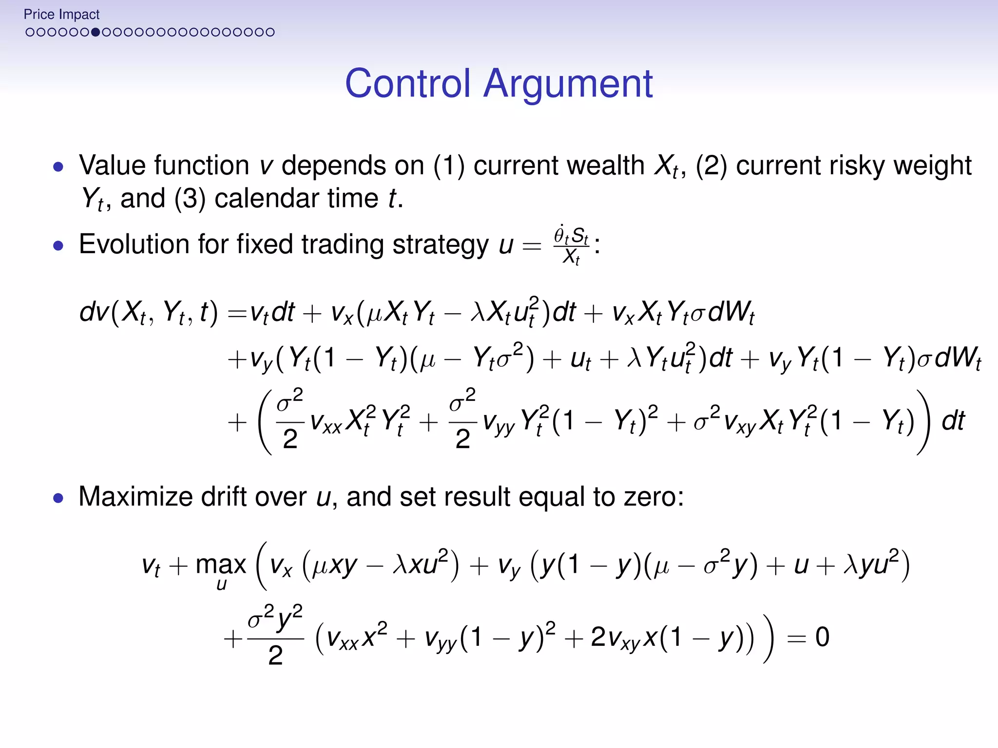
![Price Impact
Verification
Theorem
µ
If γσ 2
∈ (0, 1), then the optimal wealth turnover and equivalent safe rate are:
1 q(y )
ˆ
u (y ) = ˆ
ESRγ (u ) = β
2λ 1 − yq(y )
2
µ
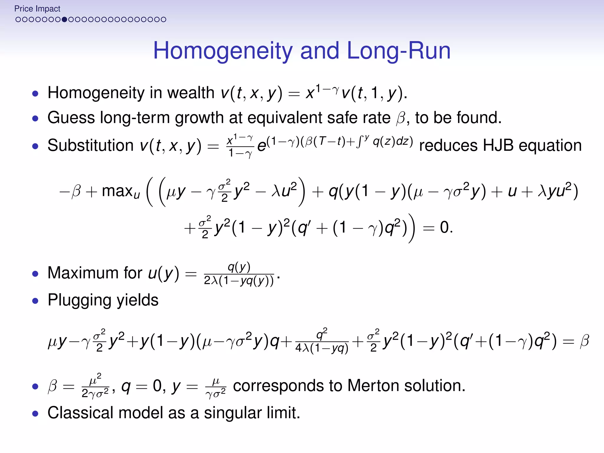
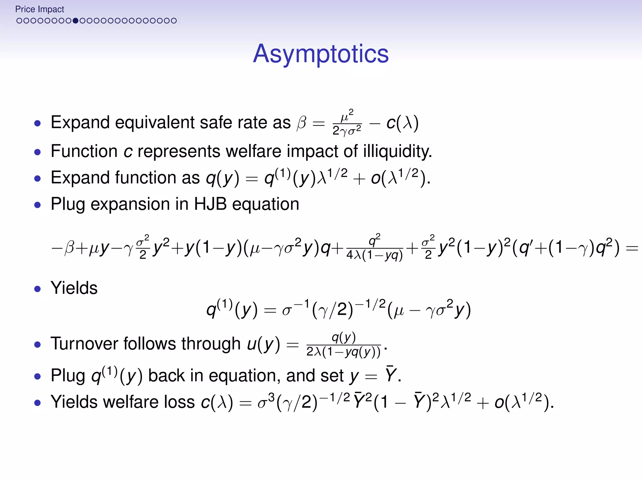
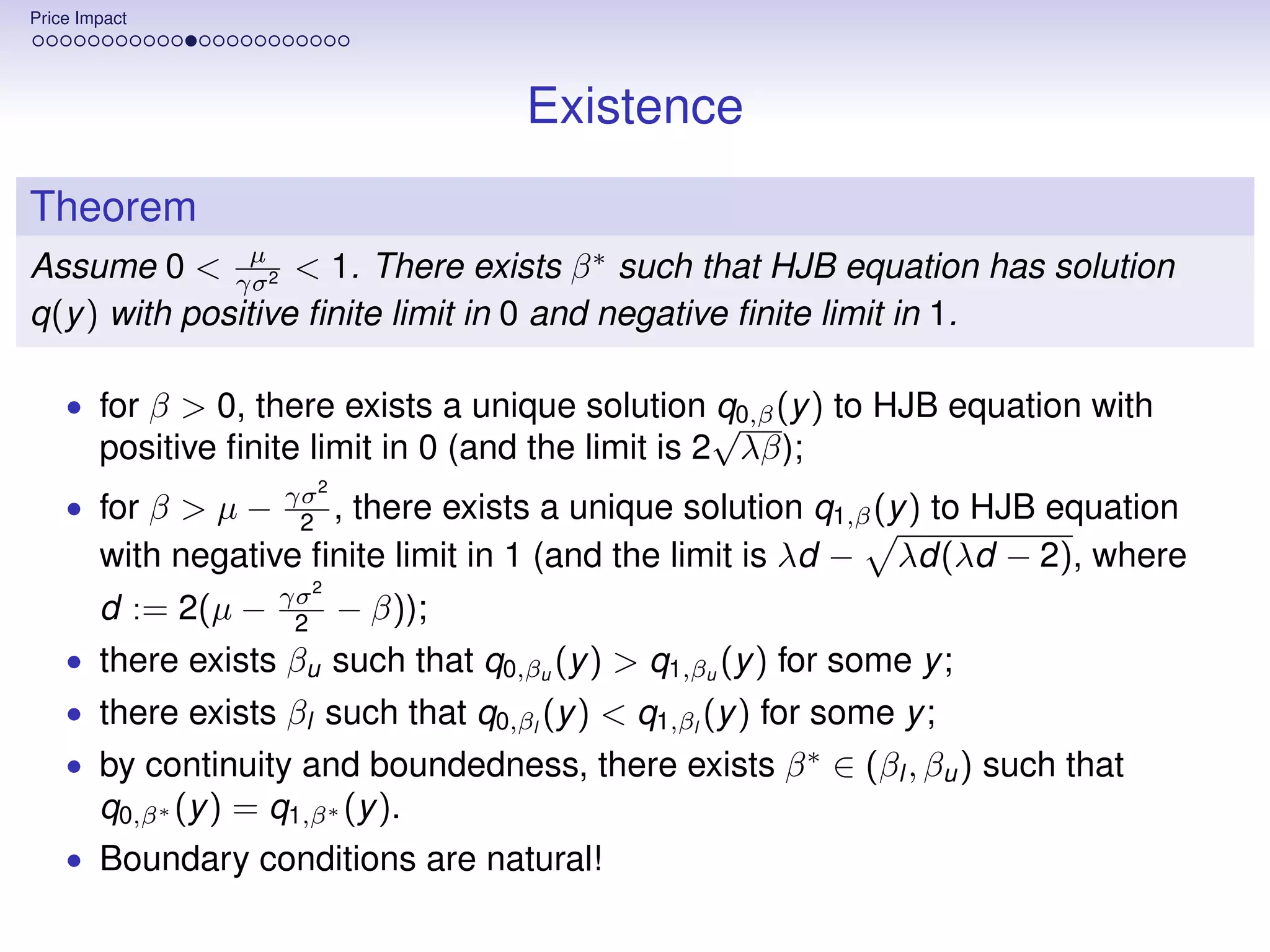
where β ∈ (0, 2γσ2 ) and q : [0, 1] → R are the unique pair that solves the ODE
2 2 2
q
−β+µy −γ σ y 2 +y (1−y )(µ−γσ 2 y )q+ 4λ(1−yq) + σ y 2 (1−y )2 (q +(1−γ)q 2 ) = 0
2 2
√
and q(0) = 2 λβ, q(1) = λd − λd(λd − 2), where d = −γσ 2 − 2β + 2µ.
• A license to solve an ODE, of Abel type.
• Function q and scalar β not explicit.
• Asymptotic expansion for λ near zero?](https://image.slidesharecdn.com/lisbonlectures-120708172712-phpapp01/75/UT-Austin-Portugal-Lectures-on-Portfolio-Choice-96-2048.jpg)
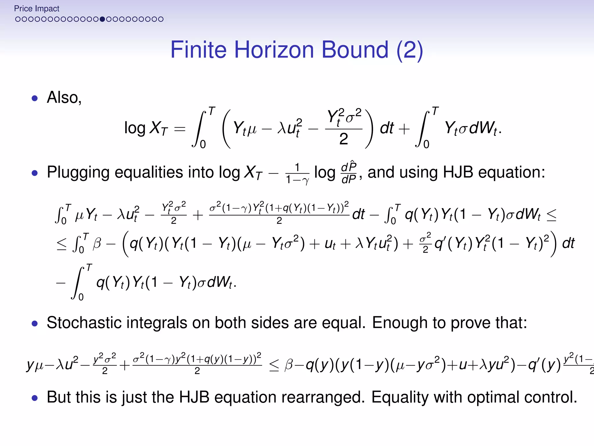
![Price Impact
Finite Horizon Bound (1)
Lemma
y ˆ
Define Q(y ) = q(z)dz. There exists a probability P, equivalent to P, such
that the terminal wealth XT of any admissible strategy satisfies:
1−γ 1 1
E[XT ] 1−γ ≤ eβT +Q(y ) EP [e−(1−γ)Q(YT ) ] 1−γ
ˆ (1)
and equality holds for the optimal strategy.
ˆ
• Define probability P as:
ˆ
dP T (1−γ)2 Ys (1+q(Ys )(1−Ys ))2 σ 2
2
T
dP
= exp 0
− 2
ds + 0
(1 − γ)Ys (1 + q(Ys )(1 − Ys ))σdWs
• It suffices to check that
1 ˆ
dP
log XT − 1−γ
log dP
≤ βT − Q(YT ) + Q(y ) .
• By self-financing condition, and Itô formula:
T Yt2 (1−Yt )2 σ 2
Q(YT ) − Q(y ) = 0
q(Yt )(Yt (1 − Yt )(µ − Yt σ 2 ) + ut + λYt ut2 ) + q (Yt ) 2
dt
T
+ q(Yt )Yt (1 − Yt )σdWt
0](https://image.slidesharecdn.com/lisbonlectures-120708172712-phpapp01/75/UT-Austin-Portugal-Lectures-on-Portfolio-Choice-98-2048.jpg)
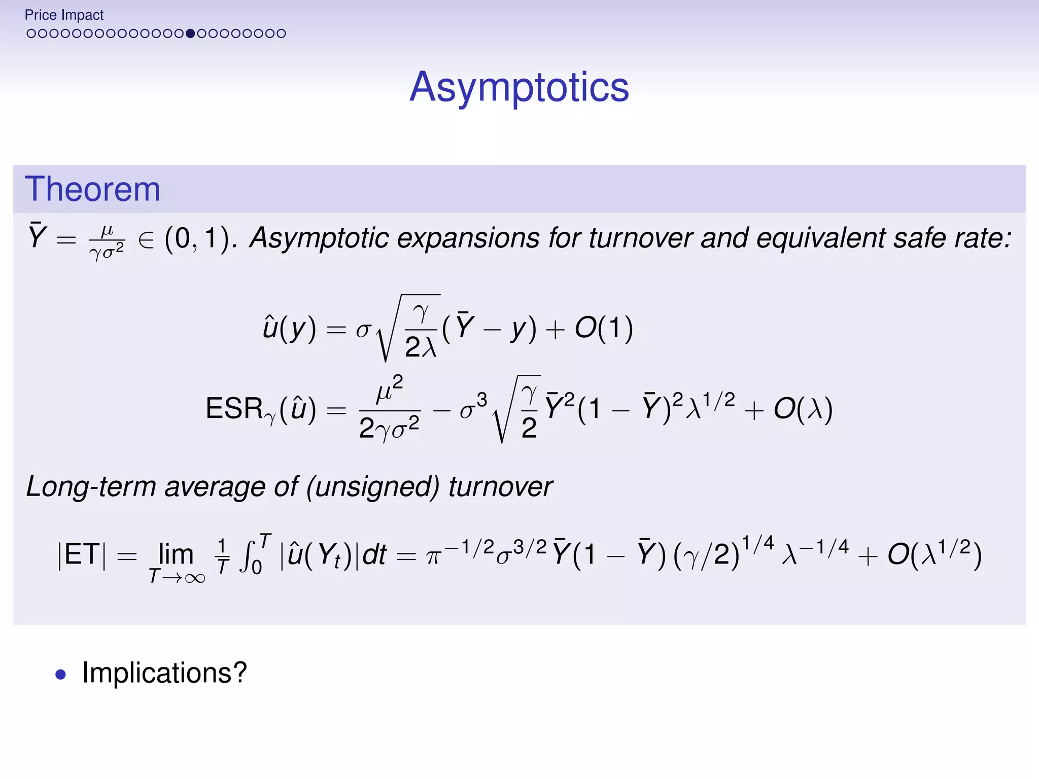
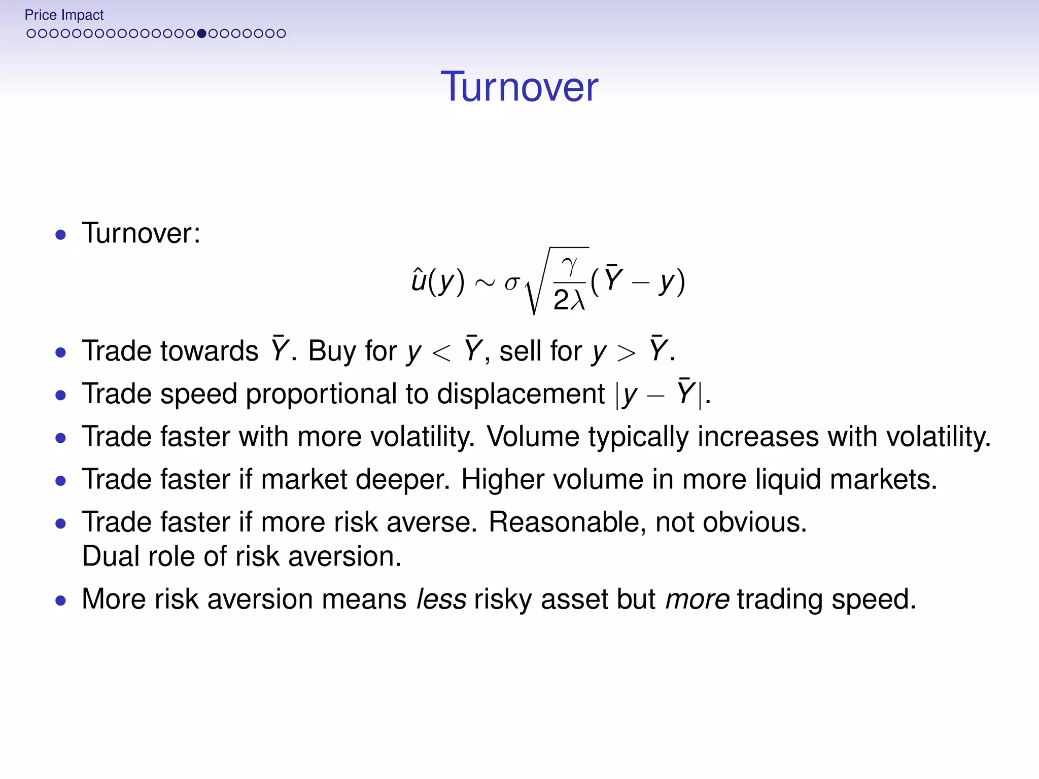
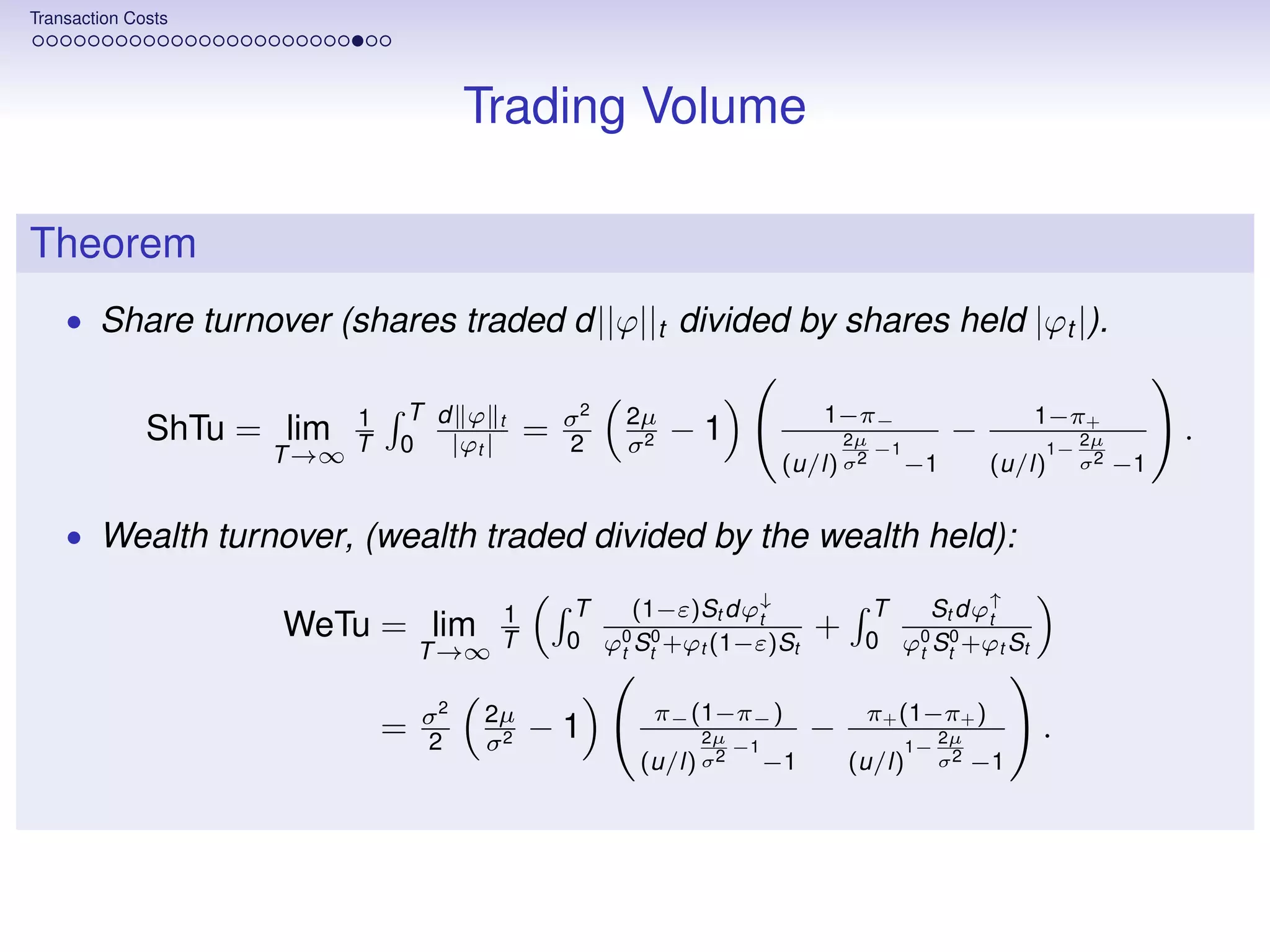
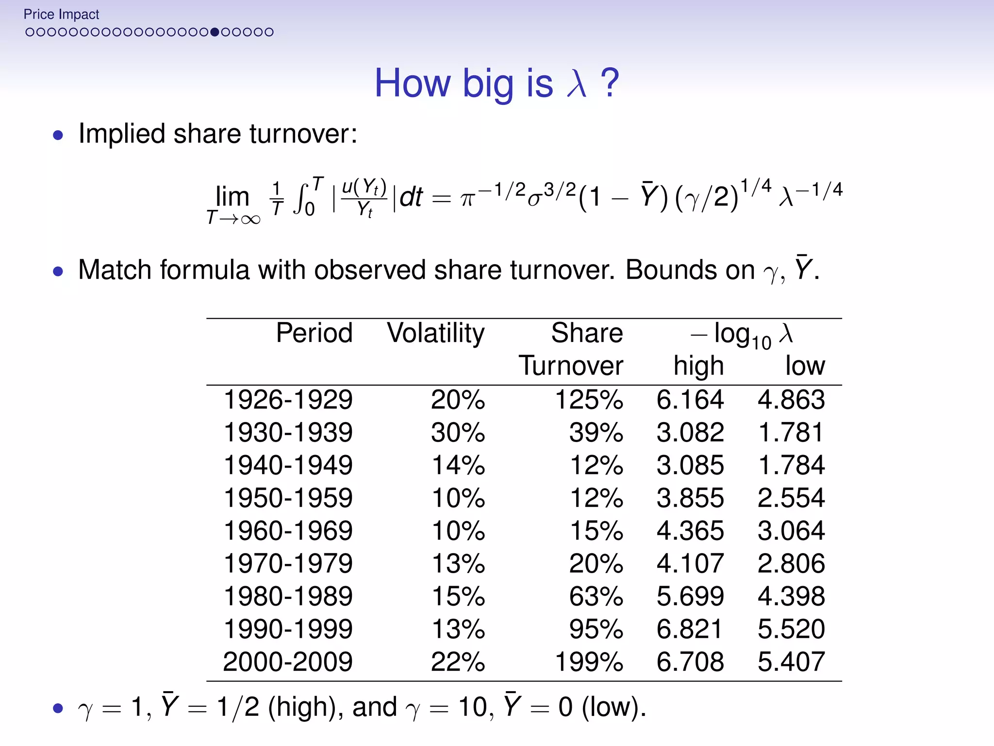
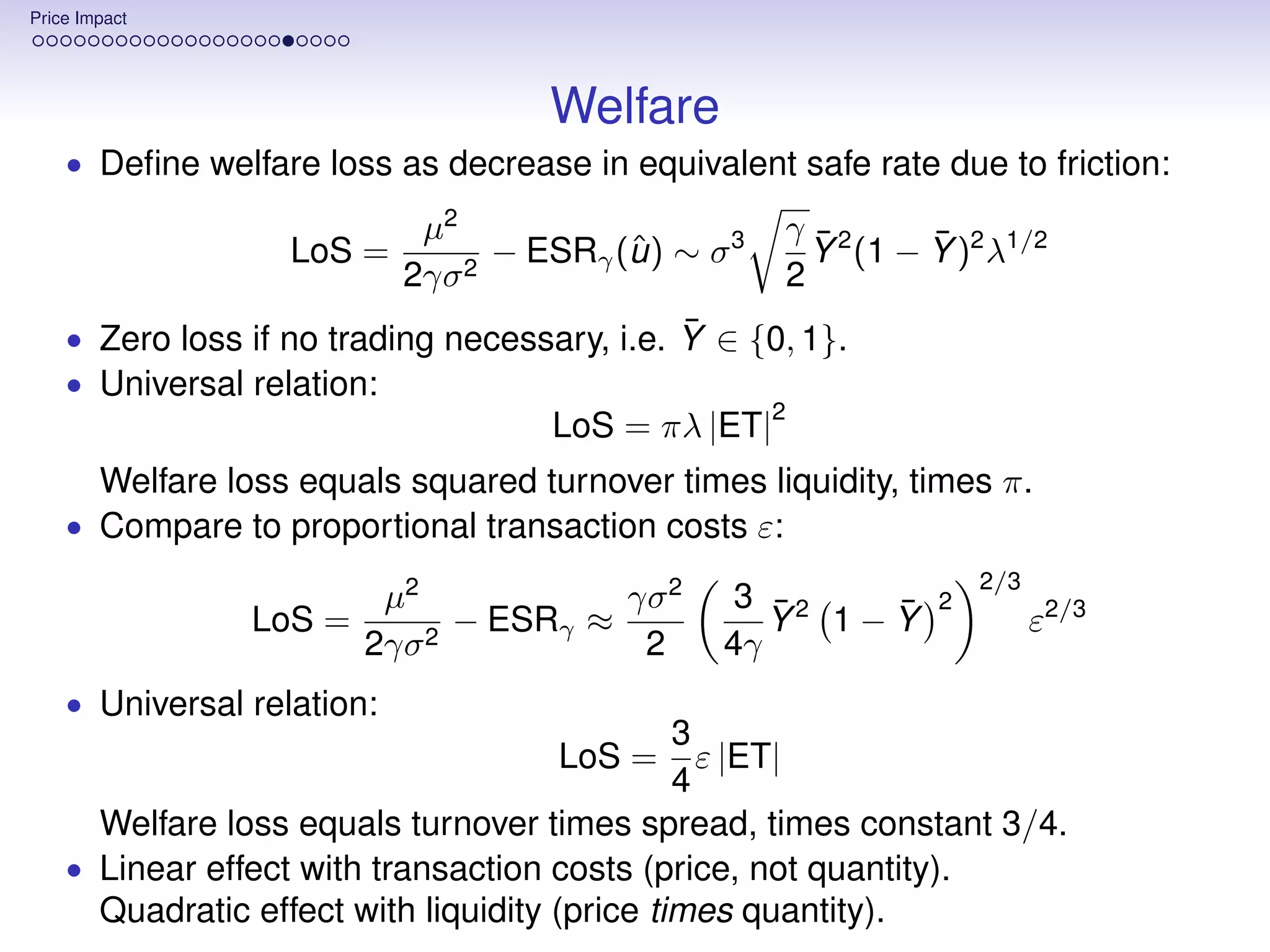
![Price Impact
Trading Volume
• Wealth turnover approximately Ornstein-Uhlenbeck:
γ 2 ¯2 ¯ γ ¯ ¯
ˆ
d ut = σ (σ Y (1 − Y )(1 − γ) − ut )dt − σ 2
ˆ Y (1 − Y )dWt
2λ 2λ
• In the following sense:
Theorem
ˆ
The process ut has asymptotic moments:
T
1 ¯ ¯
ET := lim u (Yt )dt = σ 2 Y 2 (1 − Y )(1 − γ) + o(1) ,
ˆ
T →∞ T 0
1 T 1 ¯ ¯
VT := lim (u (Yt ) − ET)2 dt = σ 3 Y 2 (1 − Y )2 (γ/2)1/2 λ1/2 + o(λ1/2 ) ,
ˆ
T →∞ T 0 2
1 ¯ ¯
QT := lim E[ u (Y ) T ] = σ 4 Y 2 (1 − Y )2 (γ/2)λ−1 + o(λ−1 )
ˆ
T →∞ T](https://image.slidesharecdn.com/lisbonlectures-120708172712-phpapp01/75/UT-Austin-Portugal-Lectures-on-Portfolio-Choice-102-2048.jpg)
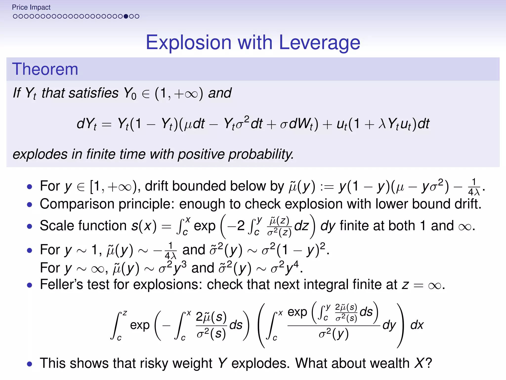
![Price Impact
Bankruptcy
• τ explosion time for Yt . Show that Xτ (ω) = 0 on ω ∈ {τ < +∞}.
• By contradiction, suppose Xt (ω) does not hit 0 on [0, τ (ω)].
T 2 T
Yt µ−λut2 − σ Yt2 dt+σ Yt dWt
XT = xe 0 2 0
.
τ τ σ2 2 τ
• If 0
Yt2 dt = ∞, then − Y dt
0 2 t
+ 0
Yt σdWt = −∞ by LLN.
τ ¯
dP τ σ2 2 τ
• If 0
Yt2 dt < ∞, define measure dP = exp − Y dt
0 2 t
+ 0
Yt σdWt
τ
• In both cases, check that 0
Yt µ − λut2 dt = −∞.
St
• 0 < (ω) < Xt (ω) < M(ω) on [0, τ (ω)], hence:
T T
T 2
limT →τ 0
Yt µ − λut2 dt < lim Mµ θt dt − λ θt2 dt
˙
T →τ 0 0
T T
θt dt
= lim θt2 dt
˙ Mµ lim 0
T
−λ 2
= −∞.
T →τ 0 T →τ ˙
θ2 dt
0 t](https://image.slidesharecdn.com/lisbonlectures-120708172712-phpapp01/75/UT-Austin-Portugal-Lectures-on-Portfolio-Choice-107-2048.jpg)
![Price Impact
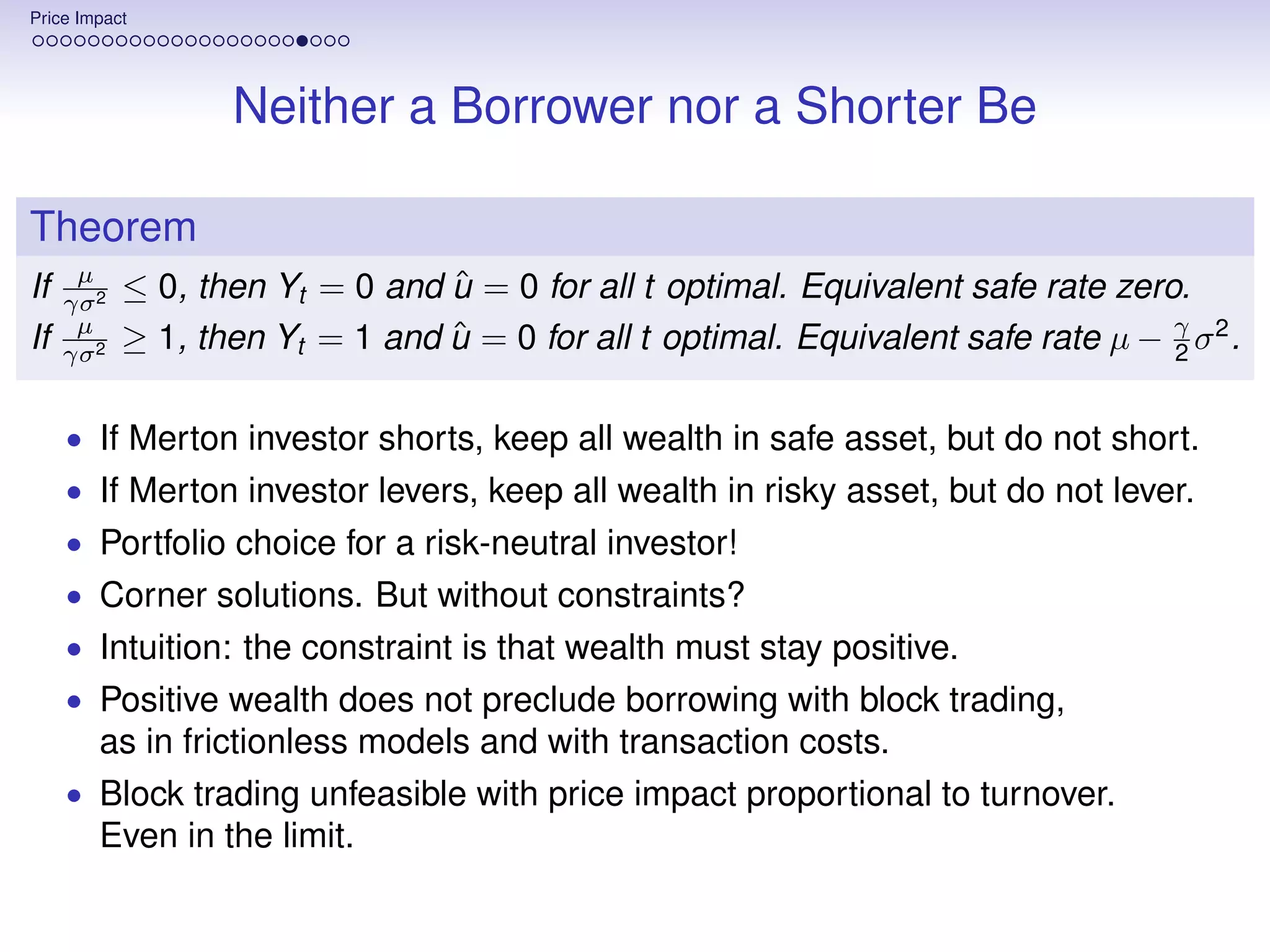
Optimality
µ
• Check that Yt ≡ 1 optimal if γσ 2
> 1.
• By Itô’s formula,
T T
1−γ
XT = x 1−γ e(1−γ) 0 (Yt µ− 1 Yt2 σ2 −λut2 )dt+(1−γ)
2 0
Yt σdWt
.
• and hence, for g(y , u) = y µ − 1 y 2 γσ 2 − λu 2 ,
2
1−γ T
E[XT ] = x 1−γ EP e
ˆ 0
(1−γ)g(Yt ,ut )dt
,
ˆ
dP T T
where dP = exp{ 0
− 1 Yt2 (1 − γ)2 σ 2 dt +
2 0
Yt (1 − γ)σdWt }.
• g(y , u) on [0, 1] × R has maximum g(1, 0) = µ − 1 γσ 2 at (1, 0).
2
• Since Yt ≡ 1 and ut ≡ 0 is admissible, it is also optimal.](https://image.slidesharecdn.com/lisbonlectures-120708172712-phpapp01/75/UT-Austin-Portugal-Lectures-on-Portfolio-Choice-108-2048.jpg)


![Lecture on nk [compatibility mode]](https://cdn.slidesharecdn.com/ss_thumbnails/lectureonnkcompatibilitymode-110825092241-phpapp01-thumbnail.jpg?width=640&height=640&fit=bounds)


