1. Efficient Projections onto the ℓ1-Ball for Learning in High Dimensions
John Duchi JDUCHI@CS.STANFORD.EDU
Google, Mountain View, CA 94043
Shai Shalev-Shwartz SHAI@TTI-C.ORG
Toyota Technological Institute, Chicago, IL, 60637
Yoram Singer SINGER@GOOGLE.COM
Tushar Chandra TUSHAR@GOOGLE.COM
Google, Mountain View, CA 94043
Abstract
We describe efficient algorithms for projecting a
vector onto the ℓ1-ball. We present two methods
for projection. The first performs exact projec-
tion in O(n) expected time, where n is the di-
mension of the space. The second works on vec-
tors k of whose elements are perturbed outside
the ℓ1-ball, projecting in O(k log(n)) time. This
setting is especially useful for online learning in
sparse feature spaces such as text categorization
applications. We demonstrate the merits and ef-
fectiveness of our algorithms in numerous batch
and online learning tasks. We show that vari-
ants of stochastic gradient projection methods
augmented with our efficient projection proce-
dures outperform interior point methods, which
are considered state-of-the-art optimization tech-
niques. We also show that in online settings gra-
dient updates with ℓ1 projections outperform the
exponentiated gradient algorithm while obtain-
ing models with high degrees of sparsity.
1. Introduction
A prevalent machine learning approach for decision and
prediction problems is to cast the learning task as penal-
ized convex optimization. In penalized convex optimiza-
tion we seek a set of parameters, gathered together in a
vector w, which minimizes a convex objective function in
w with an additional penalty term that assesses the com-
plexity of w. Two commonly used penalties are the 1-
norm and the square of the 2-norm of w. An alternative
Appearing in Proceedings of the 25th
International Conference
on Machine Learning, Helsinki, Finland, 2008. Copyright 2008
by the author(s)/owner(s).
but mathematically equivalent approach is to cast the prob-
lem as a constrained optimization problem. In this setting
we seek a minimizer of the objective function while con-
straining the solution to have a bounded norm. Many re-
cent advances in statistical machine learning and related
fields can be explained as convex optimization subject to
a 1-norm constraint on the vector of parameters w. Im-
posing an ℓ1 constraint leads to notable benefits. First, it
encourages sparse solutions, i.e a solution for which many
components of w are zero. When the original dimension
of w is very high, a sparse solution enables easier inter-
pretation of the problem in a lower dimension space. For
the usage of ℓ1-based approach in statistical machine learn-
ing see for example (Tibshirani, 1996) and the references
therein. Donoho (2006b) provided sufficient conditions for
obtaining an optimal ℓ1-norm solution which is sparse. Re-
cent work on compressed sensing (Candes, 2006; Donoho,
2006a) further explores how ℓ1 constraints can be used for
recovering a sparse signal sampled below the Nyquist rate.
The second motivation for using ℓ1 constraints in machine
learning problems is that in some cases it leads to improved
generalization bounds. For example, Ng (2004) examined
the task of PAC learning a sparse predictor and analyzed
cases in which an ℓ1 constraint results in better solutions
than an ℓ2 constraint.
In this paper we re-examine the task of minimizing a con-
vex function subject to an ℓ1 constraint on the norm of
the solution. We are particularly interested in cases where
the convex function is the average loss over a training
set of m examples where each example is represented as
a vector of high dimension. Thus, the solution itself is
a high-dimensional vector as well. Recent work on ℓ2
constrained optimization for machine learning indicates
that gradient-related projection algorithms are more effi-
cient in approaching a solution of good generalization than
second-order algorithms when the number of examples and

2. Efficient Projections onto the ℓ1-Ball for Learning in High Dimensions
the dimension are large. For instance, Shalev-Shwartz
et al. (2007) give recent state-of-the-art methods for solv-
ing large scale support vector machines. Adapting these
recent results to projection methods onto the ℓ1 ball poses
algorithmic challenges. While projections onto ℓ2 balls are
straightforward to implement in linear time with the ap-
propriate data structures, projection onto an ℓ1 ball is a
more involved task. The main contribution of this paper is
the derivation of gradient projections with ℓ1 domain con-
straints that can be performed almost as fast as gradient
projection with ℓ2 constraints.
Our starting point is an efficient method for projection onto
the probabilistic simplex. The basic idea is to show that,
after sorting the vector we need to project, it is possible to
calculate the projection exactly in linear time. This idea
was rediscovered multiple times. It was first described in
an abstract and somewhat opaque form in the work of Gafni
and Bertsekas (1984) and Bertsekas (1999). Crammer and
Singer (2002) rediscovered a similar projection algorithm
as a tool for solving the dual of multiclass SVM. Hazan
(2006) essentially reuses the same algorithm in the con-
text of online convex programming. Our starting point is
another derivation of Euclidean projection onto the sim-
plex that paves the way to a few generalizations. First we
show that the same technique can also be used for project-
ing onto the ℓ1-ball. This algorithm is based on sorting the
components of the vector to be projected and thus requires
O(n log(n)) time. We next present an improvement of the
algorithm that replaces sorting with a procedure resembling
median-search whose expected time complexity is O(n).
In many applications, however, the dimension of the feature
space is very high yet the number of features which attain
non-zero values for an example may be very small. For in-
stance, in our experiments with text classification in Sec. 7,
the dimension is two million (the bigram dictionary size)
while each example has on average one-thousand non-zero
features (the number of unique tokens in a document). Ap-
plications where the dimensionality is high yet the number
of “on” features in each example is small render our second
algorithm useless in some cases. We therefore shift gears
and describe a more complex algorithm that employs red-
black trees to obtain a linear dependence on the number
of non-zero features in an example and only logarithmic
dependence on the full dimension. The key to our con-
struction lies in the fact that we project vectors that are the
sum of a vector in the ℓ1-ball and a sparse vector—they are
“almost” in the ℓ1-ball.
In conclusion to the paper we present experimental results
that demonstrate the merits of our algorithms. We compare
our algorithms with several specialized interior point (IP)
methods as well as general methods from the literature for
solving ℓ1-penalized problems on both synthetic and real
data (the MNIST handwritten digit dataset and the Reuters
RCV1 corpus) for batch and online learning. Our projec-
tion based methods outperform competing algorithms in
terms of sparsity, and they exhibit faster convergence and
lower regret than previous methods.
2. Notation and Problem Setting
We start by establishing the notation used throughout the
paper. The set of integers 1 through n is denoted by [n].
Scalars are denoted by lower case letters and vectors by
lower case bold face letters. We use the notation w ≻ b
to designate that all of the components of w are greater
than b. We use · as a shorthand for the Euclidean norm
· 2. The other norm we use throughout the paper is the 1-
norm of the vector, v 1 =
n
i=1 |vi|. Lastly, we consider
order statistics and sorting vectors frequently throughout
this paper. To that end, we let v(i) denote the ith
order
statistic of v, that is, v(1) ≥ v(2) ≥ . . . ≥ v(n) for v ∈ Rn
.
In the setting considered in this paper we are provided with
a convex function L : Rn
→ R. Our goal is to find the
minimum of L(w) subject to an ℓ1-norm constraint on w.
Formally, the problem we need to solve is
minimize
w
L(w) s.t. w 1 ≤ z . (1)
Our focus is on variants of the projected subgradient
method for convex optimization (Bertsekas, 1999). Pro-
jected subgradient methods minimize a function L(w) sub-
ject to the constraint that w ∈ X, for X convex, by gener-
ating the sequence {w(t)
} via
w(t+1)
= ΠX w(t)
− ηt∇(t)
(2)
where ∇(t)
is (an unbiased estimate of) the (sub)gradient
of L at w(t)
and ΠX(x) = argmin y{ x − y | y ∈
X} is Euclidean projection of x onto X. In the rest of the
paper, the main algorithmic focus is on the projection step
(computing an unbiased estimate of the gradient of L(w) is
straightforward in the applications considered in this paper,
as is the modification of w(t)
by ∇(t)
).
3. Euclidean Projection onto the Simplex
For clarity, we begin with the task of performing Euclidean
projection onto the positive simplex; our derivation natu-
rally builds to the more efficient algorithms. As such, the
most basic projection task we consider can be formally de-
scribed as the following optimization problem,
minimize
w
1
2
w−v 2
2 s.t.
n
i=1
wi = z , wi ≥ 0 . (3)

3. Efficient Projections onto the ℓ1-Ball for Learning in High Dimensions
When z = 1 the above is projection onto the probabilistic
simplex. The Lagrangian of the problem in Eq. (3) is
L(w, ζ) =
1
2
w − v 2
+ θ
n
i=1
wi − z − ζ · w ,
where θ ∈ R is a Lagrange multiplier and ζ ∈ Rn
+ is a
vector of non-negative Lagrange multipliers. Differenti-
ating with respect to wi and comparing to zero gives the
optimality condition, dL
dwi
= wi − vi + θ − ζi = 0.
The complementary slackness KKT condition implies that
whenever wi > 0 we must have that ζi = 0. Thus, if
wi > 0 we get that
wi = vi − θ + ζi = vi − θ . (4)
All the non-negative elements of the vector w are tied via
a single variable, so knowing the indices of these elements
gives a much simpler problem. Upon first inspection, find-
ing these indices seems difficult, but the following lemma
(Shalev-Shwartz & Singer, 2006) provides a key tool in de-
riving our procedure for identifying non-zero elements.
Lemma 1. Let w be the optimal solution to the minimiza-
tion problem in Eq. (3). Let s and j be two indices such
that vs > vj. If ws = 0 then wj must be zero as well.
Denoting by I the set of indices of the non-zero compo-
nents of the sorted optimal solution, I = {i ∈ [n] : v(i) >
0}, we see that Lemma 1 implies that I = [ρ] for some
1 ≤ ρ ≤ n. Had we known ρ we could have simply used
Eq. (4) to obtain that
n
i=1
wi =
n
i=1
w(i) =
ρ
i=1
w(i) =
ρ
i=1
v(i) − θ = z
and therefore
θ =
1
ρ
ρ
i=1
v(i) − z . (5)
Given θ we can characterize the optimal solution for w as
wi = max {vi − θ , 0} . (6)
We are left with the problem of finding the optimal ρ, and
the following lemma (Shalev-Shwartz & Singer, 2006) pro-
vides a simple solution once we sort v in descending order.
Lemma 2. Let w be the optimal solution to the minimiza-
tion problem given in Eq. (3). Let µ denote the vector ob-
tained by sorting v in a descending order. Then, the num-
ber of strictly positive elements in w is
ρ(z, µ) = max j ∈ [n] : µj −
1
j
j
r=1
µr − z > 0 .
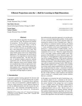
The pseudo-code describing the O(n log n) procedure for
solving Eq. (3) is given in Fig. 1.
INPUT: A vector v ∈ Rn
and a scalar z > 0
Sort v into µ : µ1 ≥ µ2 ≥ . . . ≥ µp
Find ρ = max j ∈ [n] : µj − 1
j
j
r=1
µr − z > 0
Define θ = 1
ρ
ρ
i=1
µi − z
OUTPUT: w s.t. wi = max {vi − θ , 0}
Figure 1. Algorithm for projection onto the simplex.
4. Euclidean Projection onto the ℓ1-Ball
We next modify the algorithm to handle the more general
ℓ1-norm constraint, which gives the minimization problem
minimize
w∈Rn
w − v 2
2 s.t. w 1 ≤ z . (7)
We do so by presenting a reduction to the problem of pro-
jecting onto the simplex given in Eq. (3). First, we note
that if v 1 ≤ z then the solution of Eq. (7) is w = v.
Therefore, from now on we assume that v 1 > z. In this
case, the optimal solution must be on the boundary of the
constraint set and thus we can replace the inequality con-
straint w 1 ≤ z with an equality constraint w 1 = z.
Having done so, the sole difference between the problem
in Eq. (7) and the one in Eq. (3) is that in the latter we
have an additional set of constraints, w ≥ 0. The follow-
ing lemma indicates that each non-zero component of the
optimal solution w shares the sign of its counterpart in v.
Lemma 3. Let w be an optimal solution of Eq. (7). Then,
for all i, wi vi ≥ 0.
Proof. Assume by contradiction that the claim does not
hold. Thus, there exists i for which wi vi < 0. Let ˆw
be a vector such that ˆwi = 0 and for all j = i we have
ˆwj = wj. Therefore, ˆw 1 = w 1 − |wi| ≤ z and hence
ˆw is a feasible solution. In addition,
w − v 2
2 − ˆw − v 2
2 = (wi − vi)2
− (0 − vi)2
= w2
i − 2wivi > w2
i > 0 .
We thus constructed a feasible solution ˆw which attains an
objective value smaller than that of w. This leads us to the
desired contradiction.
Based on the above lemma and the symmetry of the ob-
jective, we are ready to present our reduction. Let u be a
vector obtained by taking the absolute value of each com-
ponent of v, ui = |vi|. We now replace Eq. (7) with
minimize
β∈Rn
β − u 2
2 s.t. β 1 ≤ z and β ≥ 0 . (8)
Once we obtain the solution for the problem above we con-
struct the optimal of Eq. (7) by setting wi = sign(vi) βi.

4. Efficient Projections onto the ℓ1-Ball for Learning in High Dimensions
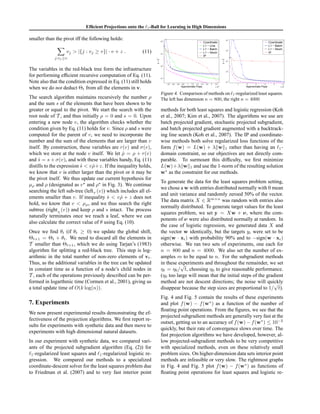
INPUT A vector v ∈ Rn
and a scalar z > 0
INITIALIZE U = [n] s = 0 ρ = 0
WHILE U = φ
PICK k ∈ U at random
PARTITION U:
G = {j ∈ U | vj ≥ vk}
L = {j ∈ U | vj < vk}
CALCULATE ∆ρ = |G| ; ∆s =
j∈G
vj
IF (s + ∆s) − (ρ + ∆ρ)vk < z
s = s + ∆s ; ρ = ρ + ∆ρ ; U ← L
ELSE
U ← G {k}
ENDIF
SET θ = (s − z)/ρ
OUTPUT w s.t. vi = max {vi − θ , 0}
Figure 2. Linear time projection onto the simplex.
5. A Linear Time Projection Algorithm
In this section we describe a more efficient algorithm for
performing projections. To keep our presentation simple
and easy to follow, we describe the projection algorithm
onto the simplex. The generalization to the ℓ1 ball can
straightforwardly incorporated into the efficient algorithm
by the results from the previous section (we simply work
in the algorithm with a vector of the absolute values of v,
replacing the solution’s components wi with sign(vi) · wi).
For correctness of the following discussion, we add an-
other component to v (the vector to be projected), which
we set to 0, thus vn+1 = 0 and v(n+1) = 0. Let us
start by examining again Lemma 2. The lemma implies
that the index ρ is the largest integer that still satisfies
v(ρ) − 1
ρ
ρ
r=1 v(r) − z > 0. After routine algebraic
manipulations the above can be rewritten in the following
somewhat simpler form:
ρ
i=1
v(i) − v(ρ) < z and
ρ+1
i=1
v(i) − v(ρ+1) ≥ z. (9)
Given ρ and v(ρ) we slightly rewrite the value θ as follows,
θ =
1
ρ


j:vj ≥v(ρ)
vj − z

 . (10)
The task of projection can thus be distilled to the task of
finding θ, which in turn reduces to the task of finding ρ and
the pivot element v(ρ). Our problem thus resembles the
task of finding an order statistic with an additional compli-
cating factor stemming from the need to compute summa-
tions (while searching) of the form given by Eq. (9). Our
efficient projection algorithm is based on a modification of
the randomized median finding algorithm (Cormen et al.,
2001). The algorithm computes partial sums just-in-time
and has expected linear time complexity.
The algorithm identifies ρ and the pivot value v(ρ) without
sorting the vector v by using a divide and conquer proce-
dure. The procedure works in rounds and on each round
either eliminates elements shown to be strictly smaller than
v(ρ) or updates the partial sum leading to Eq. (9). To do so
the algorithm maintains a set of unprocessed elements of
v. This set contains the components of v whose relation-
ship to v(ρ) we do not know. We thus initially set U = [n].
On each round of the algorithm we pick at random an in-
dex k from the set U. Next, we partition the set U into
two subsets G and L. G contains all the indices j ∈ U
whose components vj > vk; L contains those j ∈ U such
that vj is smaller. We now face two cases related to the
current summation of entries in v greater than the hypoth-
esized v(ρ) (i.e. vk). If j:vj ≥vk
(vj − vk) < z then by
Eq. (9), vk ≥ v(ρ). In this case we know that all the el-
ements in G participate in the sum defining θ as given by
Eq. (9). We can discard G and set U to be L as we still
need to further identify the remaining elements in L. If
j:vj ≥vk
(vj − vk) ≥ z then the same rationale implies
that vk < v(ρ). Thus, all the elements in L are smaller than
v(ρ) and can be discarded. In this case we can remove the
set L and vk and set U to be G {k}. The entire process
ends when U is empty.
Along the process we also keep track of the sum and the
number of elements in v that we have found thus far to
be no smaller than v(ρ), which is required in order not to
recalculate partial sums. The pseudo-code describing the
efficient projection algorithm is provided in Fig. 2. We
keep the set of elements found to be greater than v(ρ) only
implicitly. Formally, at each iteration of the algorithm we
maintain a variable s, which is the sum of the elements in
the set {vj : j ∈ U, vj ≥ v(ρ)}, and overload ρ to des-
ignate the cardinality of the this set throughout the algo-
rithm. Thus, when the algorithms exits its main while loop,
ρ is the maximizer defined in Lemma 1. Once the while
loop terminates, we are left with the task of calculating θ
using Eq. (10) and performing the actual projection. Since
j:vj ≥µρ
vj is readily available to us as the variable s, we
simply set θ to be (s − z)/ρ and perform the projection as
prescribed by Eq. (6).
Though omitted here for lack of space, we can also extend
the algorithms to handle the more general constraint that
ai|wi| ≤ z for ai ≥ 0.
6. Efficient Projection for Sparse Gradients
Before we dive into developing a new algorithm, we re-
mind the reader of the iterations the minimization algo-
rithm takes from Eq. (2): we generate a sequence {w(t)
}

5. Efficient Projections onto the ℓ1-Ball for Learning in High Dimensions
INPUT A balanced tree T and a scalar z > 0
INITIALIZE v⋆
= ∞, ρ∗
= n + 1, s∗
= z
CALL PIVOTSEARCH(root(T ), 0, 0)
PROCEDURE PIVOTSEARCH(v, ρ, s)
COMPUTE ˆρ = ρ + r(v) ; ˆs = s + σ(v)
IF ˆs < vˆρ + z // v ≥ pivot
IF v⋆
> v
v⋆
= v ; ρ⋆
= ˆρ ; s⋆
= ˆs
ENDIF
IF leafT
(v)
RETURN θ = (s⋆
− z)/ρ⋆
ENDIF
CALL PIVOTSEARCH(leftT
(v), ˆρ, ˆs)
ELSE // v < pivot
IF leafT
(v)
RETURN θ = (s⋆
− z)/ρ⋆
ENDIF
CALL PIVOTSEARCH rightT
(v), ρ, s
ENDIF
ENDPROCEDURE
Figure 3. Efficient search of pivot value for sparse feature spaces.
by iterating
w(t+1)
= ΠW w(t)
+ g(t)
where g(t)
= −ηt∇(t)
, W = {w | w 1 ≤ z} and ΠW is
projection onto this set.
In many applications the dimension of the feature space
is very high yet the number of features which attain a
non-zero value for each example is very small (see for in-
stance our experiments on text documents in Sec. 7). It is
straightforward to implement the gradient-related updates
in time which is proportional to the number of non-zero
features, but the time complexity of the projection algo-
rithm described in the previous section is linear in the di-
mension. Therefore, using the algorithm verbatim could be
prohibitively expensive in applications where the dimen-
sion is high yet the number of features which are “on” in
each example is small. In this section we describe a pro-
jection algorithm that updates the vector w(t)
with g(t)
and
scales linearly in the number of non-zero entries of g(t)
and
only logarithmically in the total number of features (i.e.
non-zeros in w(t)
).
The first step in facilitating an efficient projection for sparse
feature spaces is to represent the projected vector as a “raw”
vector v by incorporating a global shift that is applied to
each non-zero component. Specifically, each projection
step amounts to deducting θ from each component of v
and thresholding the result at zero. Let us denote by θt the
shift value used on the tth
iteration of the algorithm and by
Θt the cumulative sum of the shift values, Θt = s≤t θs.
The representation we employ enables us to perform the
step in which we deduct θt from all the elements of the
vector implicitly, adhering to the goal of performing a sub-
linear number of operations. As before, we assume that the
goal is to project onto the simplex. Equipped with these
variables, the jth
component of the projected vector after t
projected gradient steps can be written as max{vj −Θt, 0}.
The second substantial modification to the core algorithm is
to keep only the non-zero components of the weight vector
in a red-black tree (Cormen et al., 2001). The red-black tree
facilitates an efficient search for the pivot element (v(ρ)) in
time which is logarithmic in the dimension, as we describe
in the sequel. Once the pivot element is found we implic-
itly deduct θt from all the non-zero elements in our weight
vector by updating Θt. We then remove all the components
that are less than v(ρ) (i.e. less than Θt); this removal is
efficient and requires only logarithmic time (Tarjan, 1983).
The course of the algorithm is as follows. After t projected
gradient iterations we have a vector v(t)
whose non-zero el-
ements are stored in a red-black tree T and a global deduc-
tion value Θt which is applied to each non-zero component
just-in-time, i.e. when needed. Therefore, each non-zero
weight is accessed as vj − Θt while T does not contain the
zero elements of the vector. When updating v with a gradi-
ent, we modify the vector v(t)
by adding to it the gradient-
based vector g(t)
with k non-zero components. This update
is done using k deletions (removing vi from T such that
g
(t)
i = 0) followed by k re-insertions of v′
i = (vi + g
(t)
i )
into T , which takes O(k log(n)) time. Next we find in
O(log(n)) time the value of θt. Fig. 3 contains the algo-
rithm for this step; it is explained in the sequel. The last
step removes all elements of the new raw vector v(t)
+g(t)
which become zero due to the projection. This step is dis-
cussed at the end of this section.
In contrast to standard tree-based search procedure, to find
θt we need to find a pair of consecutive values in v that
correspond to v(ρ) and v(ρ+1). We do so by keeping track
of the smallest element that satisfies the left hand side of
Eq. (9) while searching based on the condition given on the
right hand side of the same equation. T is keyed on the val-
ues of the un-shifted vector vt. Thus, all the children in the
left (right) sub-tree of a node v represent values in vt which
are smaller (larger) than v. In order to efficiently find θt we
keep at each node the following information: (a) The value
of the component, simply denoted as v. (b) The number of
elements in the right sub-tree rooted at v, denoted r(v), in-
cluding the node v. (c) The sum of the elements in the right
sub-tree rooted at v, denoted σ(v), including the value v
itself. Our goal is to identify the pivot element v(ρ) and its
index ρ. In the previous section we described a simple con-
dition for checking whether an element in v is greater or
smaller than the pivot value. We now rewrite this expres-
sion yet one more time. A component with value v is not

6. Efficient Projections onto the ℓ1-Ball for Learning in High Dimensions
smaller than the pivot iff the following holds:
j:vj ≥v
vj > |{j : vj ≥ v}| · v + z . (11)
The variables in the red-black tree form the infrastructure
for performing efficient recursive computation of Eq. (11).
Note also that the condition expressed in Eq. (11) still holds
when we do not deduct Θt from all the elements in v.
The search algorithm maintains recursively the number ρ
and the sum s of the elements that have been shown to be
greater or equal to the pivot. We start the search with the
root node of T , and thus initially ρ = 0 and s = 0. Upon
entering a new node v, the algorithm checks whether the
condition given by Eq. (11) holds for v. Since ρ and s were
computed for the parent of v, we need to incorporate the
number and the sum of the elements that are larger than v
itself. By construction, these variables are r(v) and σ(v),
which we store at the node v itself. We let ˆρ = ρ + r(v)
and ˆs = s + σ(v), and with these variables handy, Eq. (11)
distills to the expression ˆs < vˆρ+z. If the inequality holds,
we know that v is either larger than the pivot or it may be
the pivot itself. We thus update our current hypothesis for
µρ and ρ (designated as v⋆
and ρ⋆
in Fig. 3). We continue
searching the left sub-tree (leftT
(v)) which includes all el-
ements smaller than v. If inequality ˆs < vˆρ + z does not
hold, we know that v < µρ, and we thus search the right
subtree (rightT
(v)) and keep ρ and s intact. The process
naturally terminates once we reach a leaf, where we can
also calculate the correct value of θ using Eq. (10).
Once we find θt (if θt ≥ 0) we update the global shift,
Θt+1 = Θt + θt. We need to discard all the elements in
T smaller than Θt+1, which we do using Tarjan’s (1983)
algorithm for splitting a red-black tree. This step is log-
arithmic in the total number of non-zero elements of vt.
Thus, as the additional variables in the tree can be updated
in constant time as a function of a node’s child nodes in
T , each of the operations previously described can be per-
formed in logarthmic time (Cormen et al., 2001), giving us
a total update time of O(k log(n)).
7. Experiments
We now present experimental results demonstrating the ef-
fectiveness of the projection algorithms. We first report re-
sults for experiments with synthetic data and then move to
experiments with high dimensional natural datasets.
In our experiment with synthetic data, we compared vari-
ants of the projected subgradient algorithm (Eq. (2)) for
ℓ1-regularized least squares and ℓ1-regularized logistic re-
gression. We compared our methods to a specialized
coordinate-descent solver for the least squares problem due
to Friedman et al. (2007) and to very fast interior point
0.2 0.4 0.6 0.8 1 1.2 1.4 1.6 1.8 2 2.2
x 10
8
10
−1
10
0
10
1
10
2
Approximate Flops
f−f
*
Coordinate
L1 − Line
L1 − Batch
L1 − Stoch
IP
1 2 3 4 5 6
x 10
9
10
−1
10
0
10
1
10
2
10
3
Approximate Flops
f−f
*
Coordinate
L1 − Batch
L1 − Stoch
IP
Figure 4. Comparison of methods on ℓ1-regularized least squares.
The left has dimension n = 800, the right n = 4000
methods for both least squares and logistic regression (Koh
et al., 2007; Kim et al., 2007). The algorithms we use are
batch projected gradient, stochastic projected subgradient,
and batch projected gradient augmented with a backtrack-
ing line search (Koh et al., 2007). The IP and coordinate-
wise methods both solve regularized loss functions of the
form f(w) = L(w) + λ w 1 rather than having an ℓ1-
domain constraint, so our objectives are not directly com-
parable. To surmount this difficulty, we first minimize
L(w)+λ w 1 and use the 1-norm of the resulting solution
w∗
as the constraint for our methods.
To generate the data for the least squares problem setting,
we chose a w with entries distributed normally with 0 mean
and unit variance and randomly zeroed 50% of the vector.
The data matrix X ∈ Rm×n
was random with entries also
normally distributed. To generate target values for the least
squares problem, we set y = Xw + ν, where the com-
ponents of ν were also distributed normally at random. In
the case of logistic regression, we generated data X and
the vector w identically, but the targets yi were set to be
sign(w · xi) with probability 90% and to −sign(w · xi)
otherwise. We ran two sets of experiments, one each for
n = 800 and n = 4000. We also set the number of ex-
amples m to be equal to n. For the subgradient methods
in these experiments and throughout the remainder, we set
ηt = η0/
√
t, choosing η0 to give reasonable performance.
(η0 too large will mean that the initial steps of the gradient
method are not descent directions; the noise will quickly
disappear because the step sizes are proportional to 1/
√
t).
Fig. 4 and Fig. 5 contain the results of these experiments
and plot f(w) − f(w∗
) as a function of the number of
floating point operations. From the figures, we see that the
projected subgradient methods are generally very fast at the
outset, getting us to an accuracy of f(w) − f(w∗
) ≤ 10−2
quickly, but their rate of convergence slows over time. The
fast projection algorithms we have developed, however, al-
low projected-subgradient methods to be very competitive
with specialized methods, even on these relatively small
problem sizes. On higher-dimension data sets interior point
methods are infeasible or very slow. The rightmost graphs
in Fig. 4 and Fig. 5 plot f(w) − f(w∗
) as functions of
floating point operations for least squares and logistic re-

7. Efficient Projections onto the ℓ1-Ball for Learning in High Dimensions
0.5 1 1.5 2 2.5 3 3.5 4 4.5 5 5.5
x 10
8
10
−4
10
−3
10
−2
10
−1
Approximate Flops
f−f
*
L1 − Line
L1 − Batch
L1 − Stoch
IP
1 2 3 4 5 6 7 8
x 10
9
10
−5
10
−4
10
−3
10
−2
10
−1
Approximate Flops
f−f
*
L1 − Batch
L1 − Stoch
IP
Figure 5. Comparison of methods on ℓ1-regularized logistic re-
gression. The left has dimension n = 800, the right n = 4000
gression with dimension n = 4000. These results indicate
that in high dimensional feature spaces, the asymptotically
faster convergence of IP methods is counteracted by their
quadratic dependence on the dimension of the space.
We also ran a series of experiments on two real datasets
with high dimensionality: the Reuters RCV1 Cor-
pus (Lewis et al., 2004) and the MNIST handwritten digits
database. The Reuters Corpus has 804,414 examples; with
simple stemming and stop-wording, there are 112,919 uni-
gram features and 1,946,684 bigram features. With our pre-
processing, the unigrams have a sparsity of 1.2% and the bi-
grams have sparsity of .26%. We performed ℓ1-constrained
binary logistic regression on the CCAT category from
RCV1 (classifying a document as corporate/industrial) us-
ing unigrams in a batch setting and bigrams in an online set-
ting. The MNIST dataset consists of 60,000 training exam-
ples and a 10,000 example test set and has 10-classes; each
image is a gray-scale 28×28 image, which we represent as
xi ∈ R784
. Rather than directly use the input xi, however,
we learned weights wj using the following Kernel-based
“similarity” function for each class j ∈ {1, . . . , 10}:
k(x, j) =
i∈S
wjiσjiK(xi, x), σji =
1 if yi = j
−1 otherwise.
In the above, K is a Gaussian kernel function, so that
K(x, y) = exp(− x − y 2
/25), and S is a 2766 element
support set. We put an ℓ1 constraint on each wj, giving us
the following multiclass objective with dimension 27,660:
minimizew
1
m
m
i=1 log 1 + r=yi
ek(xi,r)−k(xi,yi)
s.t. wj 1 ≤ z, wj 0.
(12)
As a comparison to our projected subgradient methods on
real data, we used a method known in the literature as either
entropic descent, a special case of mirror descent (Beck &
Teboulle, 2003), or exponentiated gradient (EG) (Kivinen
& Warmuth, 1997). EG maintains a weight vector w sub-
ject to the constraint that i wi = z and w 0; it can
easily be extended to work with negative weights under a
1-norm constraint by maintaining two vectors w+
and w−
.
We compare against EG since it works well in very high di-
0 20 40 60 80 100 120
10
−3
10
−2
10
−1
Time (CPU seconds)
f−f
*
L1 − Stoch
L1 − Full
EG − Full
EG − Stoch
0 50 100 150 200 250 300 350 400 450
10
−4
10
−3
10
−2
10
−1
Time (CPU seconds)
f−f
*
L1 − 1
EG − 1
L1 − 100
EG − 100
Figure 6. EG and projected subgradient methods on RCV1.
mensional spaces, and it very quickly identifies and shrinks
weights for irrelevant features (Kivinen & Warmuth, 1997).
At every step of EG we update
w
(t+1)
i =
w
(t)
i exp −ηt∇if(w(t)
)
Zt
(13)
where Zt normalizes so that i w
(t+1)
i = z and ∇if
denotes the ith
entry of the gradient of f, the function
to be minimized. EG can actually be viewed as a pro-
jected subgradient method using generalized relative en-
tropy (D(x y) = i xi log xi
yi
− xi + yi) as the distance
function for projections (Beck & Teboulle, 2003). We can
replace ∇if with ˆ∇if in Eq. (13), an unbiased estimator
of the gradient of f, to get stochastic EG. A step size ηt ∝
1/
√
t guarantees a convergence rate of O( log n/T). For
each experiment with EG, however, we experimented with
learning rates proportional to 1/t, 1/
√
t, and constant, as
well as different initial step-sizes; to make EG as competi-
tive as possible, we chose the step-size and rate for which
EG performed best on each individual test..
Results for our batch experiments learning a logistic classi-
fier for CCAT on the Reuters corpus can be seen in Fig. 6.
The figure plots the binary logistic loss of the different al-
gorithms minus the optimal log loss as a function of CPU
time. On the left side Fig. 6, we used projected gradient
descent and stochastic gradient descent using 25% of the
training data to estimate the gradient, and we used the al-
gorithm of Fig. 2 for the projection steps. We see that ℓ1-
projections outperform EG both in terms of convergence
speed and empirical log-loss. On the right side of the fig-
ure, we performed stochastic descent using only 1 training
example or 100 training examples to estimate the gradient,
using Fig. 3 to project. When the gradient is sparse, up-
dates for EG are O(k) (where k is the number of non-zeros
in the gradient), so EG has a run-time advantage over ℓ1-
projections when the gradient is very sparse. This advan-
tage can be seen in the right side of Fig. 6.
For MNIST, with dense features, we ran a similar series
of tests to those we ran on the Reuters Corpus. We plot
the multiclass logistic loss from Eq. (12) over time (as a
function of the number gradient evaluations) in Fig. 7. The
left side of Fig. 7 compares EG and gradient descent using

8. Efficient Projections onto the ℓ1-Ball for Learning in High Dimensions
2 4 6 8 10 12 14 16 18 20
10
−1
10
0
Gradient Evaluations
f−f
*
EG
L1
50 100 150 200 250 300 350 400
10
−1
10
0
Stochastic Subgradient Evaluations
f−f
*
EG
L1
Figure 7. MNIST multiclass logistic loss as a function of the
number of gradient steps. The left uses true gradients, the right
stochastic subgradients.
0 1 2 3 4 5 6 7 8
x 10
5
0.5
1
1.5
2
2.5
3
3.5
x 10
5
Training Examples
CumulativeLoss
EG − CCAT
EG − ECAT
L1 − CCAT
L1 − ECAT
0 1 2 3 4 5 6 7 8
x 10
5
0
1
2
3
4
5
6
7
Training Examples
%Sparsity
% of Total Features
% of Total Seen
Figure 8. Online learning of bigram classifier on RCV1. Left is
the cumulative loss, right shows sparsity over time.
the true gradient while the right figure compares stochas-
tic EG and stochastic gradient descent using only 1% of
the training set to estimate the gradient. On top of outper-
forming EG in terms of convergence rate and loss, the ℓ1-
projection methods also gave sparsity, zeroing out between
10 and 50% of the components of each class vector wj in
the MNIST experiments, while EG gives no sparsity.
As a last experiment, we ran an online learning test on
the RCV1 dataset using bigram features, comparing ℓ1-
projections to using decreasing step sizes given by Zinke-
vich (2003) to exponential gradient updates. The ℓ1-
projections are computationally feasible because of algo-
rithm 3, as the dimension of our feature space is nearly 2
million (using the expected linear-time algorithm of Fig. 2
takes 15 times as long to compute the projection for the
sparse updates in online learning). We selected the bound
on the 1-norm of the weights to give the best online re-
gret of all our experiments (in our case, the bound was
100). The results of this experiment are in Fig. 8. The
left figure plots the cumulative log-loss for the CCAT and
ECAT binary prediction problems as a function of the num-
ber of training examples, while the right hand figure plots
the sparsity of the ℓ1-constrained weight vector both as a
function of the dimension and as a function of the number
of features actually seen. The ℓ1-projecting learner main-
tained an active set with only about 5% non-zero compo-
nents; the EG updates have no sparsity whatsoever. Our on-
line ℓ1-projections outperform EG updates in terms of the
online regret (cumulative log-loss), and the ℓ1-projection
updates also achieve a classification error rate of 11.9%
over all the examples on the CCAT task and 14.9% on
ECAT (versus more than 15% and 20% respectively for
EG).
Acknowledgments
We thank the anonymous reviewers for their helpful and
insightful comments.
References
Beck, A., & Teboulle, M. (2003). Mirror descent and nonlinear
projected subgradient methods for convex optimization. Opera-
tions Research Letters, 31, 167–175.
Bertsekas, D. (1999). Nonlinear programming. Athena Scien-
tific.
Candes, E. J. (2006). Compressive sampling. Proc. of the Int.
Congress of Math., Madrid, Spain.
Cormen, T. H., Leiserson, C. E., Rivest, R. L., & Stein, C.
(2001). Introduction to algorithms. MIT Press.
Crammer, K., & Singer, Y. (2002). On the learnability and de-
sign of output codes for multiclass problems. Machine Learning,
47.
Donoho, D. (2006a). Compressed sensing. Technical Report,
Stanford University.
Donoho, D. (2006b). For most large underdetermined systems of
linear equations, the minimal ℓ1-norm solution is also the spars-
est solution. Comm. Pure Appl. Math. 59.
Friedman, J., Hastie, T., & Tibshirani, R. (2007). Pathwise co-
ordinate optimization. Annals of Applied Statistics, 1, 302–332.
Gafni, E., & Bertsekas, D. P. (1984). Two-metric projection
methods for constrained optimization. SIAM Journal on Control
and Optimization, 22, 936–964.
Hazan, E. (2006). Approximate convex optimization by online
game playing. Unpublished manuscript.
Kim, S.-J., Koh, K., Lustig, M., Boyd, S., & Gorinevsky, D.
(2007). An interior-point method for large-scale ℓ1-regularized
least squares. IEEE Journal on Selected Topics in Signal Pro-
cessing, 4, 606–617.
Kivinen, J., & Warmuth, M. (1997). Exponentiated gradient ver-
sus gradient descent for linear predictors. Information and Com-
putation, 132, 1–64.
Koh, K., Kim, S.-J., & Boyd, S. (2007). An interior-point
method for large-scale ℓ1-regularized logistic regression. Jour-
nal of Machine Learning Research, 8, 1519–1555.
Lewis, D., Yang, Y., Rose, T., & Li, F. (2004). Rcv1: A new
benchmark collection for text categorization research. Journal
of Machine Learning Research, 5, 361–397.
Ng, A. (2004). Feature selection, l1 vs. l2 regularization, and
rotational invariance. Proceedings of the Twenty-First Interna-
tional Conference on Machine Learning.
Shalev-Shwartz, S., & Singer, Y. (2006). Efficient learning of
label ranking by soft projections onto polyhedra. Journal of Ma-
chine Learning Research, 7 (July), 1567–1599.
Shalev-Shwartz, S., Singer, Y., & Srebro, N. (2007). Pegasos:
Primal estimated sub-gradient solver for SVM. Proceedings of
the 24th International Conference on Machine Learning.
Tarjan, R. E. (1983). Data structures and network algorithms.
Society for Industrial and Applied Mathematics.
Tibshirani, R. (1996). Regression shrinkage and selection via
the lasso. J. Royal. Statist. Soc B., 58, 267–288.
Zinkevich, M. (2003). Online convex programming and general-
ized infinitesimal gradient ascent. Proceedings of the Twentieth
International Conference on Machine Learning.