Download to read offline


![An Adaptive Metric
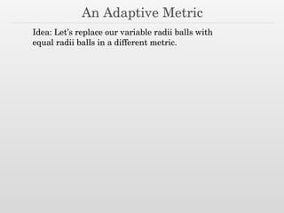
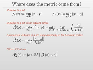
Idea: Let’s replace our variable radii balls with
equal radii balls in a different metric.
(t)
: [0, a] :! Rd](https://image.slidesharecdn.com/osu16sampling-160613132440/85/Some-Thoughts-on-Sampling-8-320.jpg)
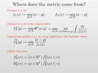
![An Adaptive Metric
Idea: Let’s replace our variable radii balls with
equal radii balls in a different metric.
(t)
: [0, a] :! Rd
len( ) :=
Z a
0
k 0
(t)kL
dt](https://image.slidesharecdn.com/osu16sampling-160613132440/85/Some-Thoughts-on-Sampling-9-320.jpg)
![An Adaptive Metric
Idea: Let’s replace our variable radii balls with
equal radii balls in a different metric.
(t)
: [0, a] :! Rd
len( ) :=
Z a
0
k 0
(t)kL
dt](https://image.slidesharecdn.com/osu16sampling-160613132440/85/Some-Thoughts-on-Sampling-10-320.jpg)
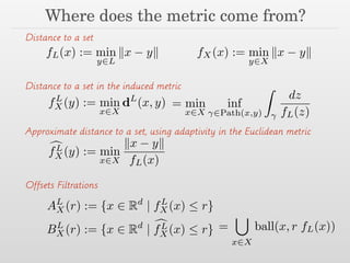
![An Adaptive Metric
Idea: Let’s replace our variable radii balls with
equal radii balls in a different metric.
(t)
: [0, a] :! Rd
len( ) :=
Z a
0
k 0
(t)kL
dt
=
Z a
0
k 0
(t)k
fL( (t))
dt](https://image.slidesharecdn.com/osu16sampling-160613132440/85/Some-Thoughts-on-Sampling-11-320.jpg)
![An Adaptive Metric
Idea: Let’s replace our variable radii balls with
equal radii balls in a different metric.
(t)
: [0, a] :! Rd
len( ) :=
Z a
0
k 0
(t)kL
dt
=
Z a
0
k 0
(t)k
fL( (t))
dt
=
Z
dz
fL(z)](https://image.slidesharecdn.com/osu16sampling-160613132440/85/Some-Thoughts-on-Sampling-12-320.jpg)
![An Adaptive Metric
Idea: Let’s replace our variable radii balls with
equal radii balls in a different metric.
(t)
: [0, a] :! Rd
len( ) :=
Z a
0
k 0
(t)kL
dt
=
Z a
0
k 0
(t)k
fL( (t))
dt
=
Z
dz
fL(z)
dL
(x, y) := inf
2Path(x,y)
len( )
The metric induced by L.](https://image.slidesharecdn.com/osu16sampling-160613132440/85/Some-Thoughts-on-Sampling-13-320.jpg)
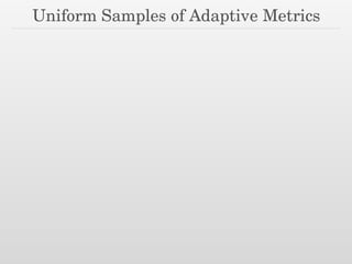
![An Adaptive Metric
Idea: Let’s replace our variable radii balls with
equal radii balls in a different metric.
(t)
: [0, a] :! Rd
len( ) :=
Z a
0
k 0
(t)kL
dt
=
Z a
0
k 0
(t)k
fL( (t))
dt
=
Z
dz
fL(z)
dL
(x, y) := inf
2Path(x,y)
len( )
The metric induced by L.
Coming up: Adaptive samples correspond to uniform samples
in the metric induced by L.](https://image.slidesharecdn.com/osu16sampling-160613132440/85/Some-Thoughts-on-Sampling-14-320.jpg)


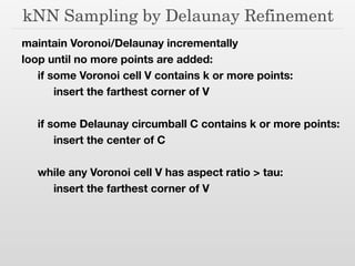
![kNN Sampling by Delaunay Refinement
maintain Voronoi/Delaunay incrementally
loop until no more points are added:
if some Voronoi cell V contains k or more points:
insert the farthest corner of V
!
if some Delaunay circumball C contains k or more points:
insert the center of C
!
while any Voronoi cell V has aspect ratio > tau:
insert the farthest corner of V
Based on Sparse Voronoi Refinement [Hudson et al ’06]](https://image.slidesharecdn.com/osu16sampling-160613132440/85/Some-Thoughts-on-Sampling-83-320.jpg)


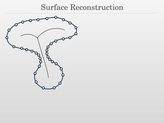
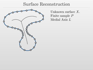
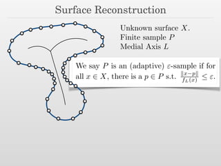
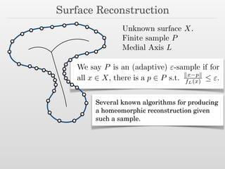
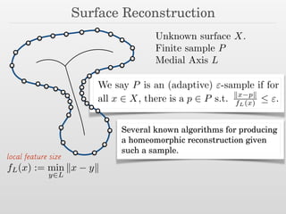
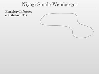
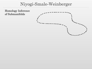
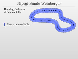
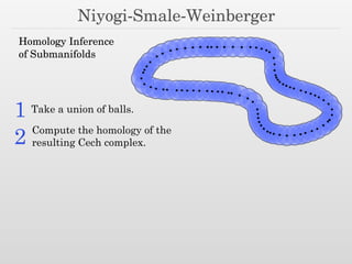
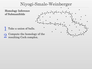
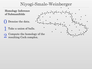
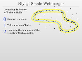
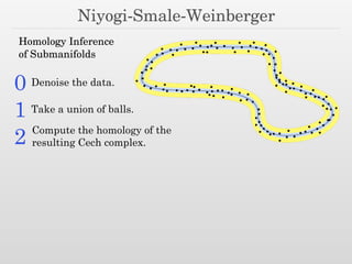
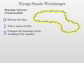
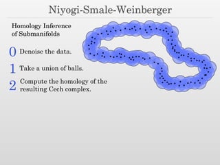
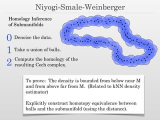
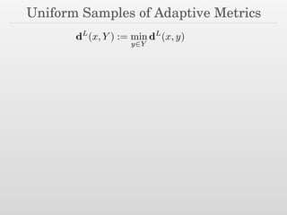
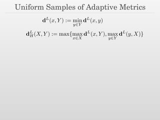
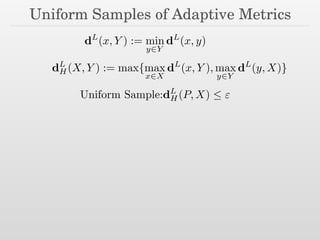
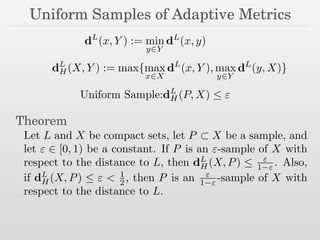
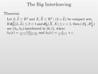
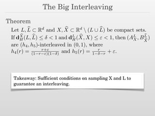
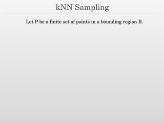
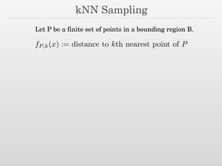
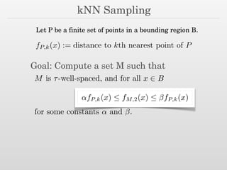
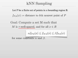
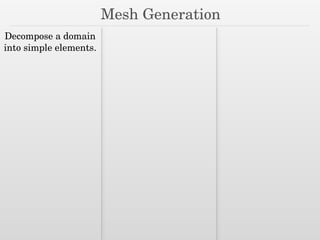
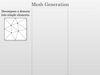
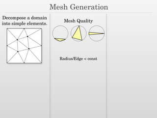
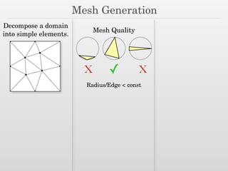
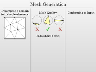
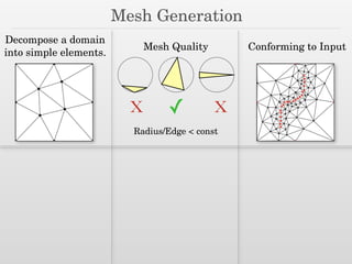
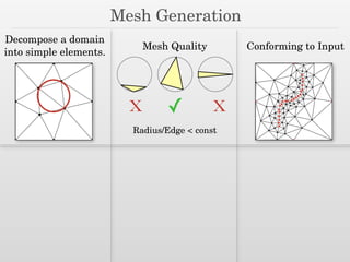
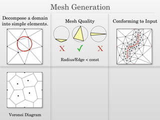
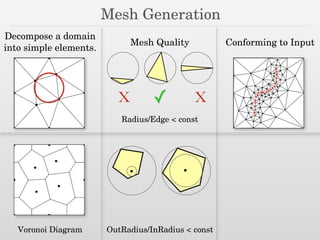
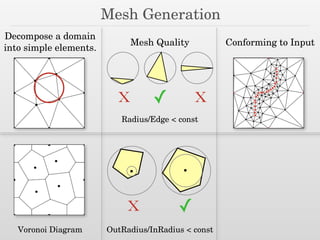
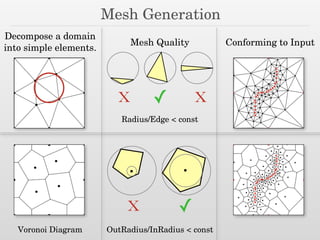
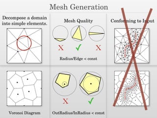
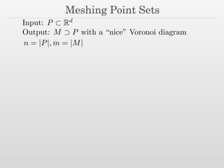
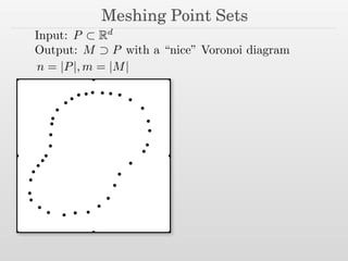
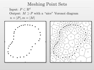
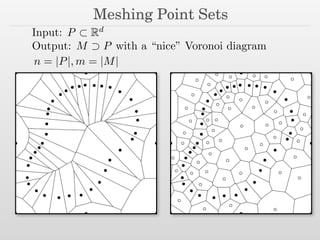
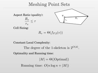
The document discusses surface reconstruction and adaptive sampling techniques in the context of geometric data analysis. It highlights the importance of homology inference, critical point theory, and properties of distance functions in effective reconstruction and sampling strategies. Additionally, it addresses mesh generation and the quality criteria for decomposing a domain into simple elements.