Downloaded 13 times
![INTRODUCTION
4 Ws
• Who
- Dr David Hurley (then a PhD student )
Dr Mark Nixon & Dr John Carter [1]
• When
- year 2001
• Where
- University of Southampton
• Why
- Objective was to reduce dimensionality of
pattern space yet maintain discriminatory power for
classification and invariant description in context of Ear
Biometrics.
3](https://image.slidesharecdn.com/forcefieldtransformation-131115063831-phpapp02/75/Force-Field-Transformation-3-2048.jpg)
![POINT & GROUP OPERATORS
• Point Operators : Basic operation in IP where each pixel value
is replaced with a new value obtained by
carrying out certain operations on the
previous pixel value.[2]
• Group Operators : Same as Point Operator but here the new
value of the pixel is determined by past
values of its neighbouring pixels. [2]
4](https://image.slidesharecdn.com/forcefieldtransformation-131115063831-phpapp02/75/Force-Field-Transformation-4-2048.jpg)
![POINT & GROUP OPERATORS
• Types of Point Operators [2]
1. Histogram Operations for Brightness/contrast control
2. Thresholding Operator for finding object of interest in an
image if its brightness level is known
• Types of Group Operators – used for filtering [2]
1. Template Convolution uses weighted coefficient template
2. Averaging Operator – equally weighted (1 or 1/9)
coefficient template
3. Gaussian Averaging Operator – template coefficient are
values set by Gaussian relationship
4. Median & Mode Operator – use statistical relationship
5. Anisotropic Diffusion – uses Heat Flow eq for calculating
the coefficients of the template.
6. Force Field Transform – ‘Today’s Topic of Discussion’!!!
5](https://image.slidesharecdn.com/forcefieldtransformation-131115063831-phpapp02/75/Force-Field-Transformation-5-2048.jpg)
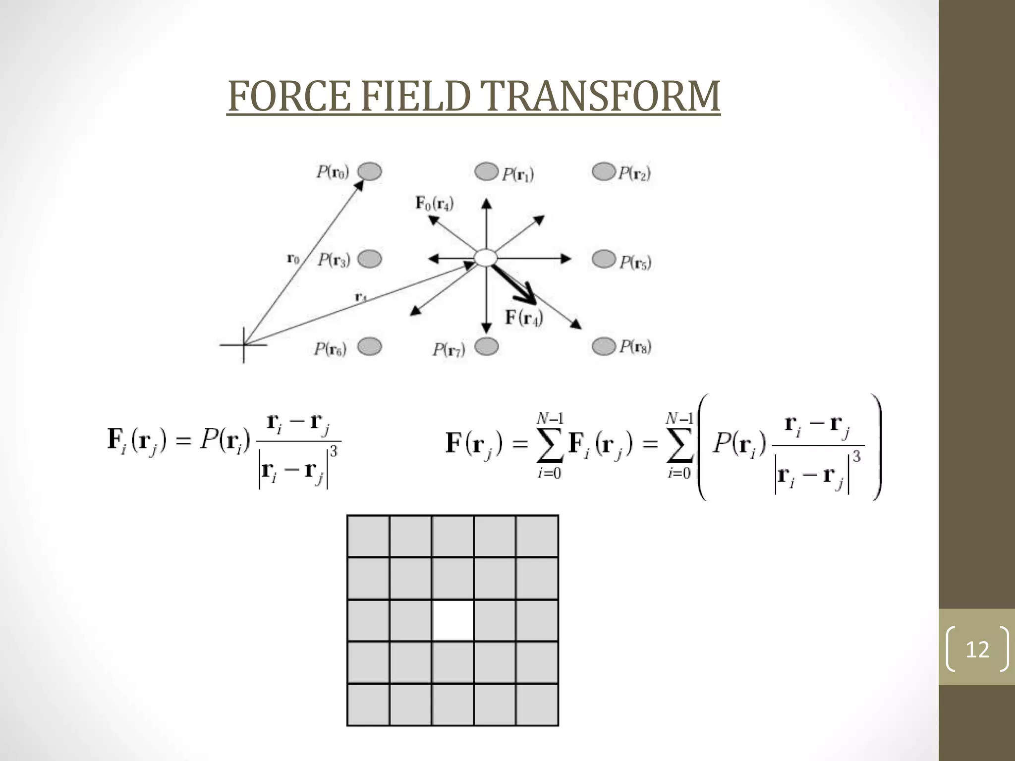
![FORCE FIELD TRANSFORM
(For Unit Test Pixel) [1]
7](https://image.slidesharecdn.com/forcefieldtransformation-131115063831-phpapp02/75/Force-Field-Transformation-7-2048.jpg)
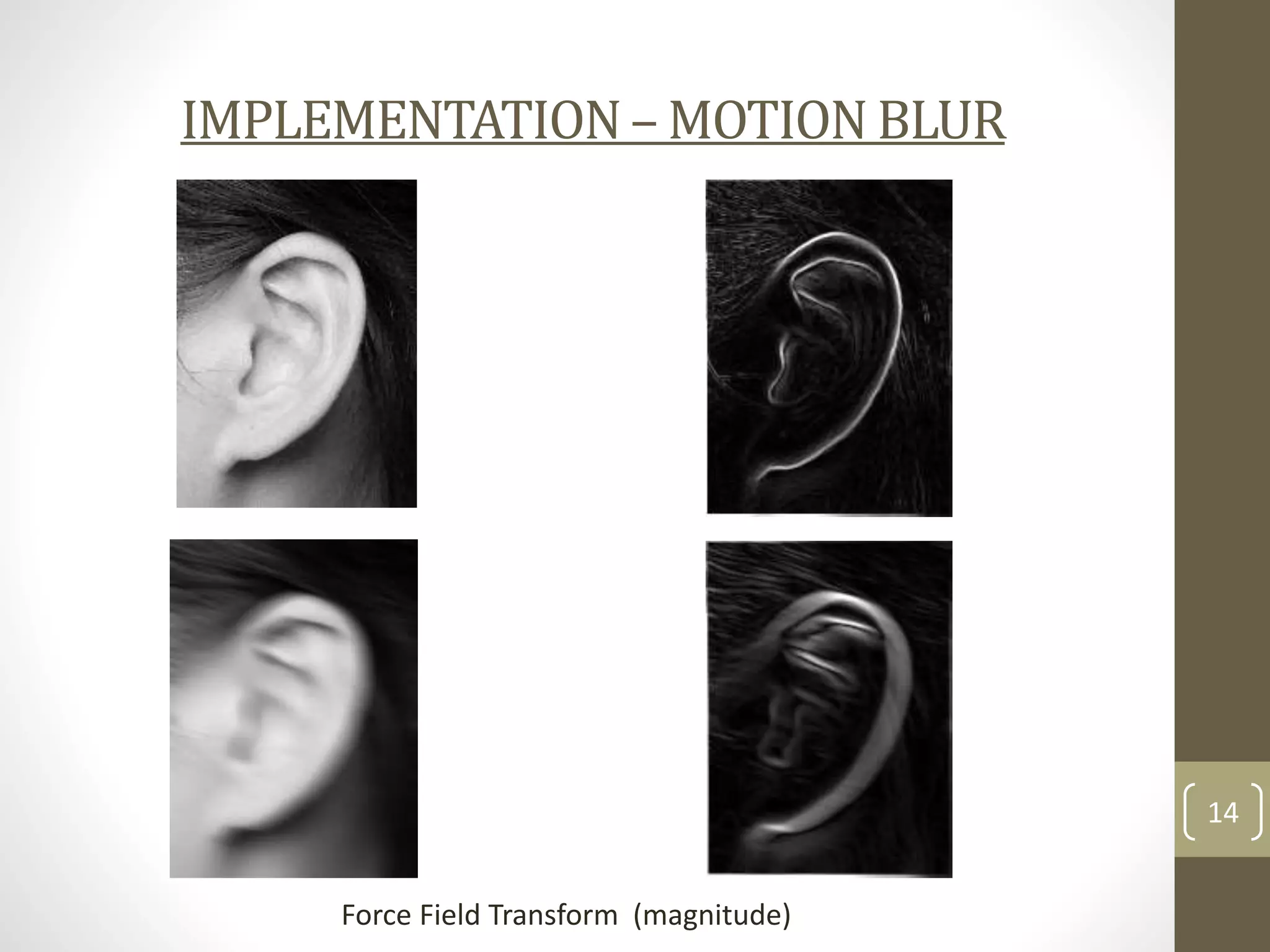
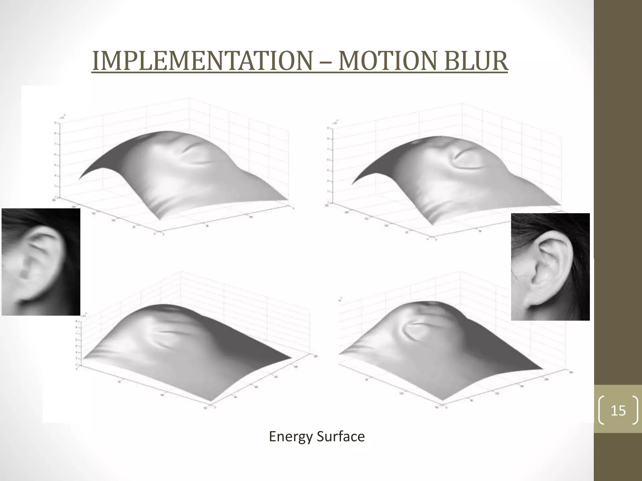
![FORCE FIELD TRANSFORM
Fig 3. Original Image
Force Field
(Magnitude)
Fig 4. Array of
Test Pixels
Field lines, channels
and wells
Potential Ridges and wells are obtained by placing 50 test
pixels which generate field lines when iterated over time [3]
8](https://image.slidesharecdn.com/forcefieldtransformation-131115063831-phpapp02/75/Force-Field-Transformation-8-2048.jpg)
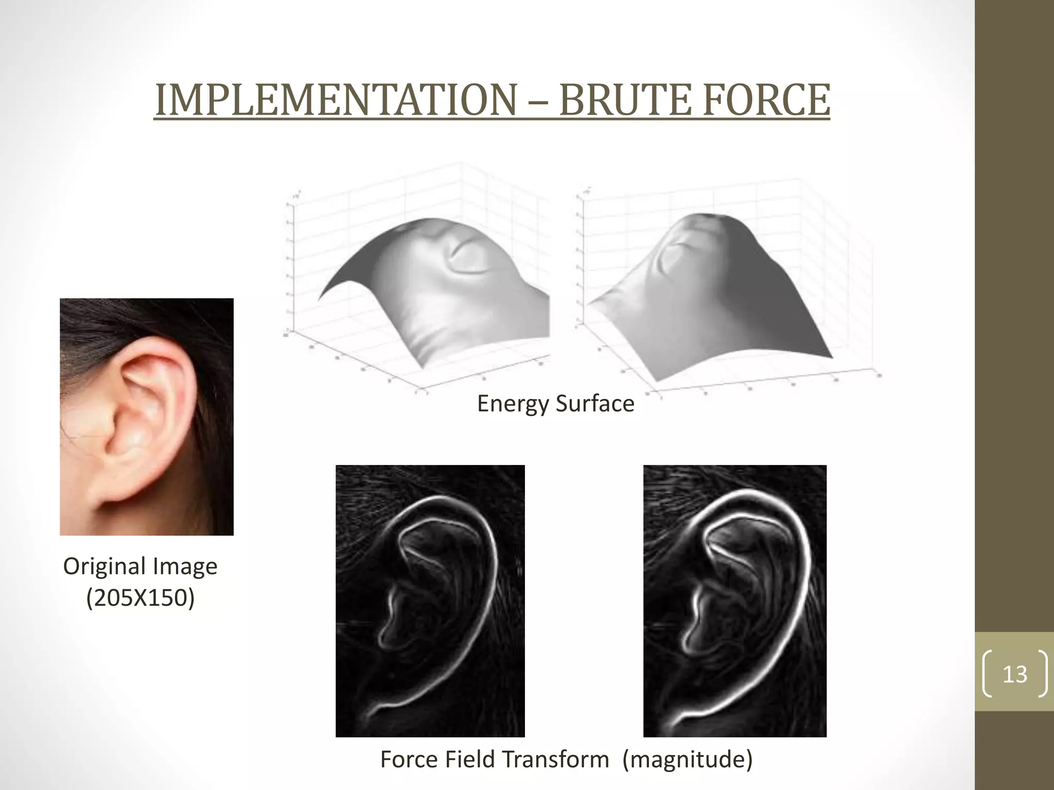
![MATHEMATICAL MODEL – BRUTE FORCE
Here each pixel is transformed using the defining
equations for Force and energy. [1]
Or equivalently matrix multiplication as shown below
could be used
4X4 pixel image
where,
10](https://image.slidesharecdn.com/forcefieldtransformation-131115063831-phpapp02/75/Force-Field-Transformation-10-2048.jpg)
![MATHEMATICAL MODEL – FREQUENCY
DOMAIN ANALYSIS
Here a MxN pixel image is convolved with a Force Field
matrix for a unit pixel.[1]
The advantage of working in frequency domain is that
the computational time reduces from O (N^2) to O(N log N).
11](https://image.slidesharecdn.com/forcefieldtransformation-131115063831-phpapp02/75/Force-Field-Transformation-11-2048.jpg)
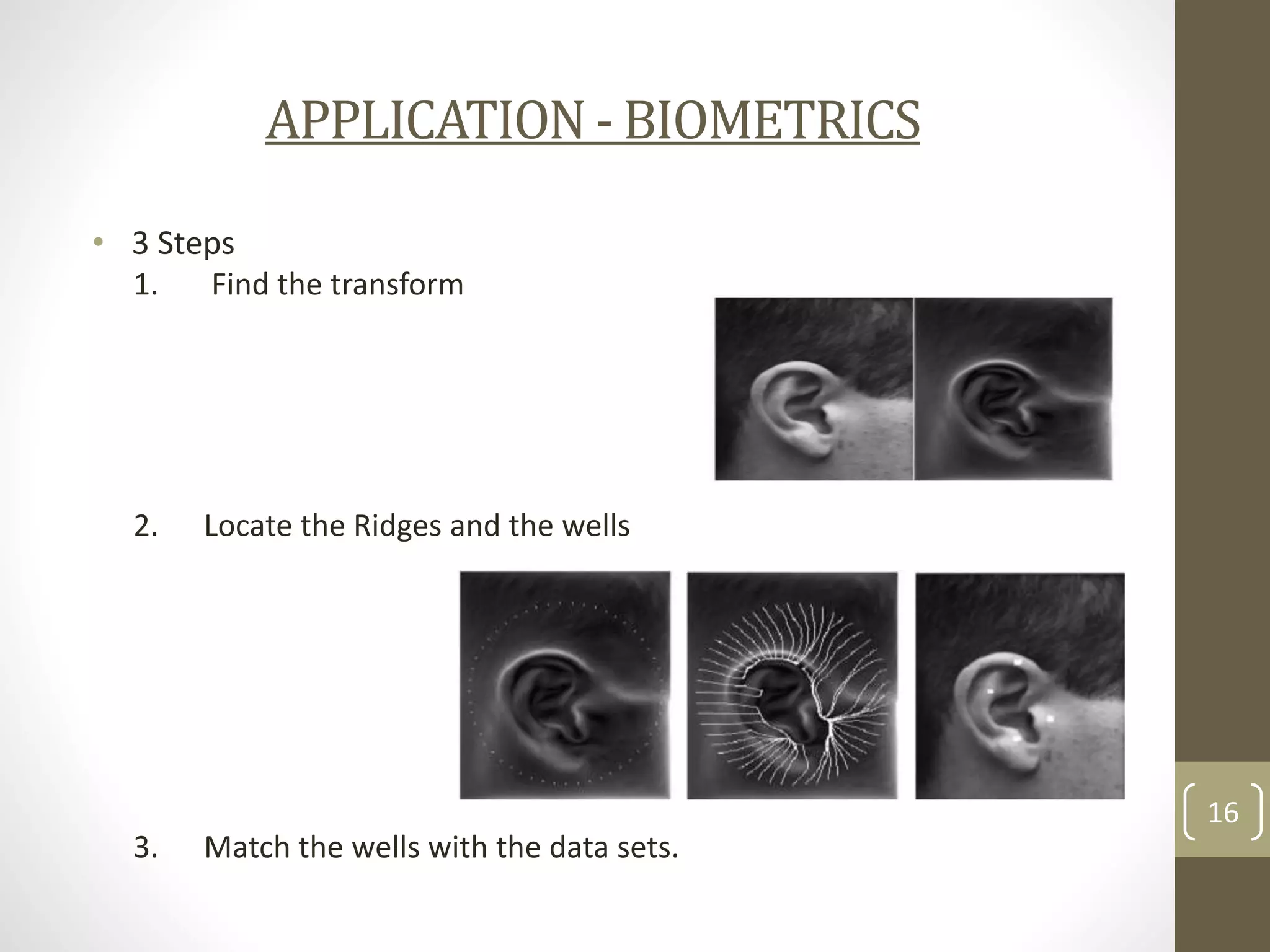
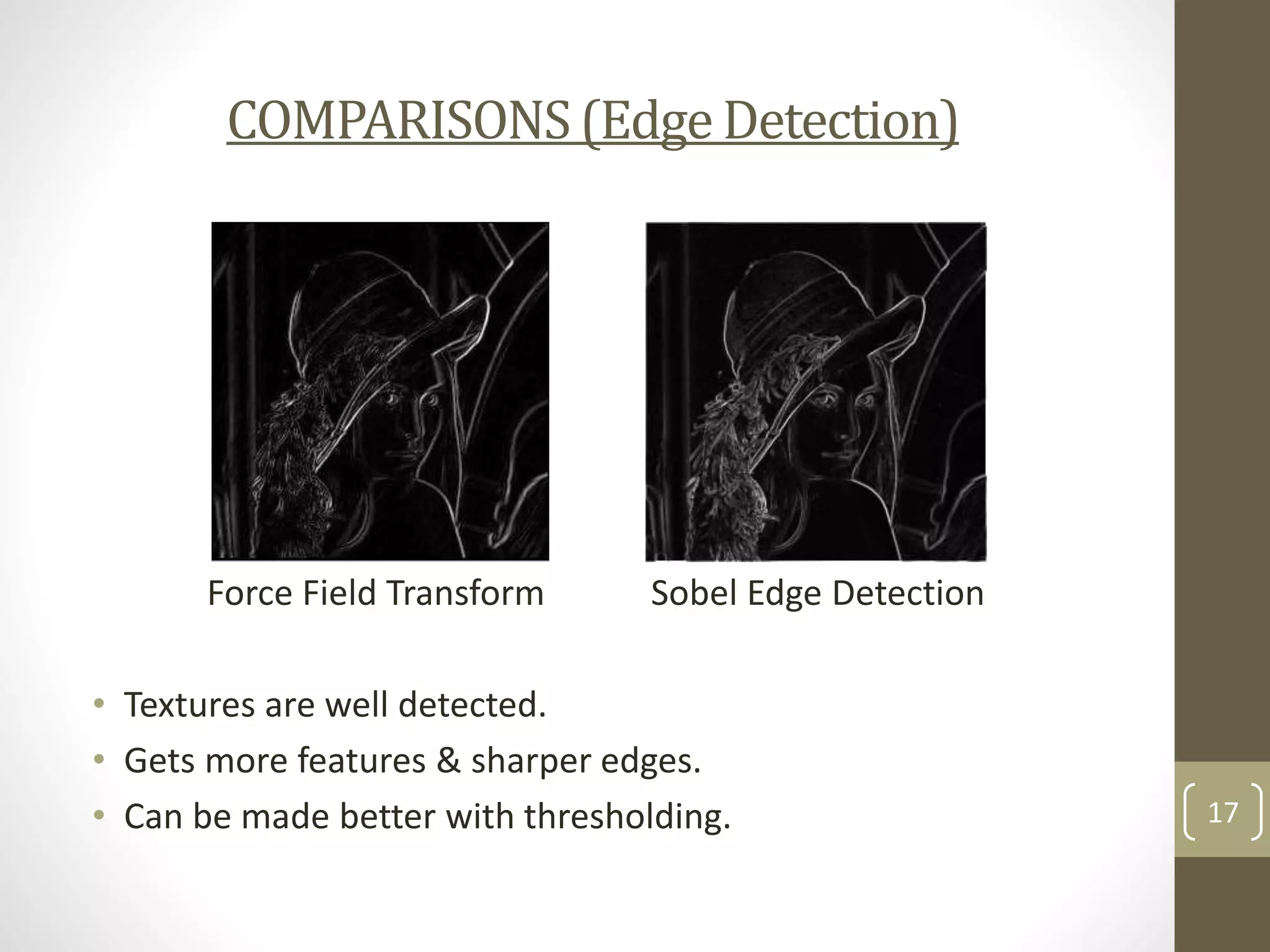

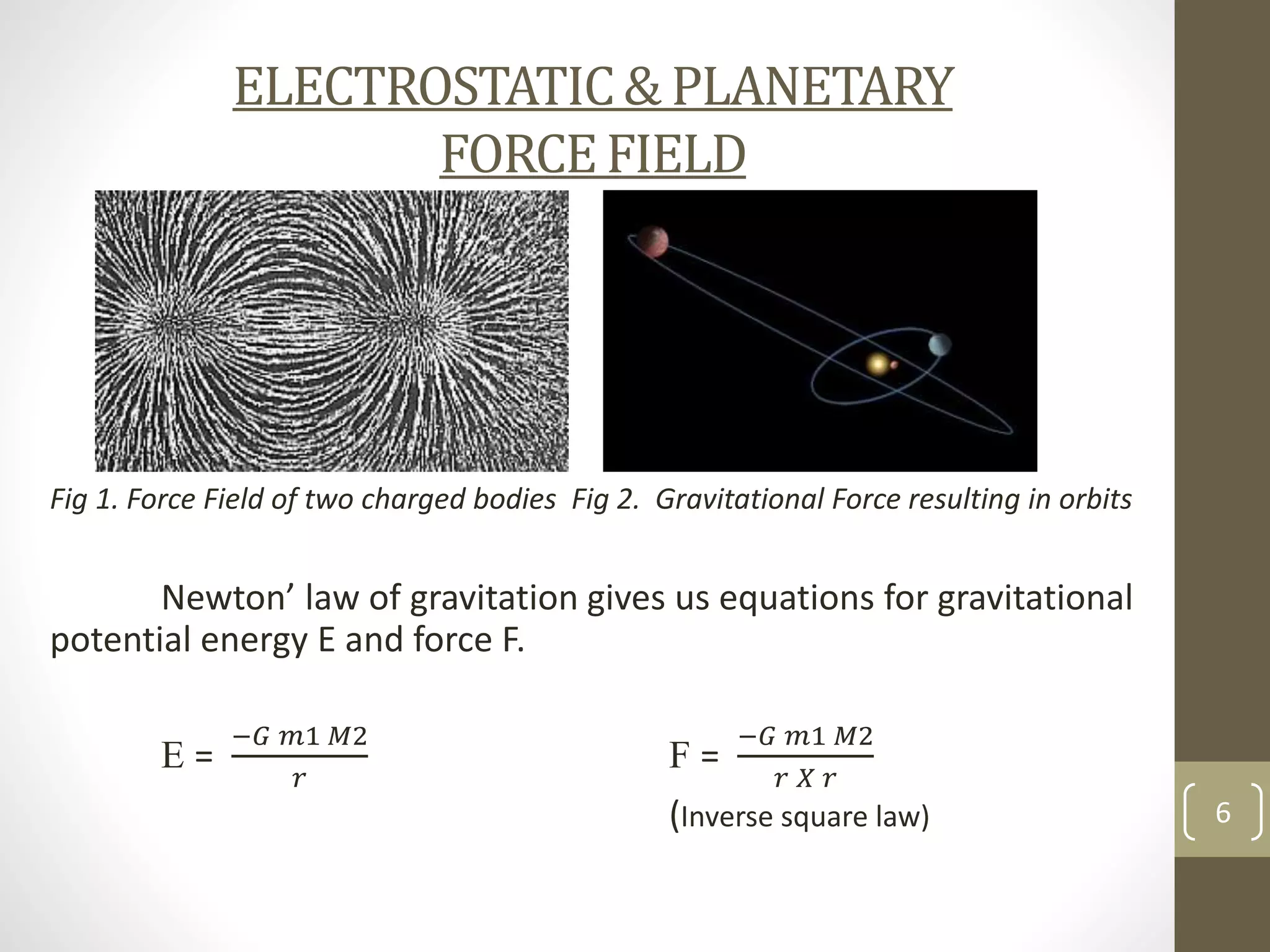
The document summarizes force field transforms, a technique for dimensionality reduction and feature extraction in images. It was developed by Dr. David Hurley in 2001 for use in ear biometrics. The technique models each pixel as a charged particle and calculates the force and energy fields. This maps the image to an energy surface highlighting ridges and wells for use as features. It offers improved edge detection over Sobel and was shown to achieve 99.2% accuracy in ear identification, outperforming other techniques. The document covers the mathematical models, implementations, applications in biometrics, advantages of being robust to distortion, and contributions of related ear biometric research.