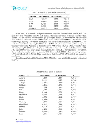
The study estimates global solar radiation (GSR) for 53 locations using various machine learning methods, including elm, svr, knn, lr, and nu-svr. The nu-svr method demonstrated the highest accuracy, with an RMSE of 1.4972 mj/m2, while lr performed the worst. The research emphasizes the efficacy of machine learning techniques in modeling solar radiation, highlighting the potential of leveraging satellite data for improved estimations.
![International Journal of Thales Engineering Sciences (JTHES)
ISSN (print): 2149-5173
7 | P a g e
www.thalespublisher.com
Estimation of Global Solar Radiation by Using Machine Learning
Methods
Mehmet Bolat
Engineering Faculty/Siirt University
Mehmet Şahin
Engineering Faculty/Siirt University
ABSTRACT
In this study, global solar radiation (GSR) was estimated based on 53 locations by using ELM, SVR,
KNN, LR and NU-SVR methods. Methods were trained with a two-year data set and accuracy of the
mentioned methods was tested with a one-year data set. The data set of each year was consisting of 12
months. Whereas the values of month, altitude, latitude, longitude, vapour pressure deficit and land surface
temperature were used as input for developing models, GSR was obtained as output. Values of vapour
pressure deficit and land surface temperature were taken from radiometry of NOAA-AVHRR satellite.
Estimated solar radiation data were compared with actual data that were obtained from meteorological
stations. According to statistical results, most successful method was NU-SVR method. The RMSE and
MBE values of NU-SVR method were found to be 1,4972 MJ/m2
and 0,2652 MJ/m2
, respectively. R value
was 0,9728. Furthermore, worst prediction method was LR. For other methods, RMSE values were
changing between 1,7746 MJ/m2
and 2,4546 MJ/m2
. It can be seen from the statistical results that ELM,
SVR, k-NN and NU-SVR methods can be used for estimation of GSR.
Keywords: Global Solar Radiation, NU-SVR
1 INTRODUCTION
The world has abundant solar energy resources. So that we need essentially to search sources of
energy. Nowadays, climate change is increasing effects on human life. It shows us; why we must work
more and more about this. One of them is GSR that is measured by a pyranometer but its installation is a
very costly, takes long time and unusual way, especially in the developing countries. As mentioned,
meteorological data based on many various factor and for each point, it cannot be measure easily. Cause of
all these reason, it is modeled by some methods and it is estimated by this models. Estimation of daily GSR
by the sunshine based models (Linear, Quadratic and Cubic) has been made and compared. The comparison
results showed that the cubic model is equivalent to the quadratic model and the most constructive statistical
results are given by the quadratic model [1]. Clearness index-beam transmittance numerical correlation was
proposed using measured ambient temperature and relative humidity data to estimate hourly solar radiation
[2]. Many researchers developed the correlations to predict the mean monthly diffuse solar radiation.
However, most of these are based on regression analyses which are limited in accuracy and the number of
parameters they can handle effectively [3,4]. The major drawback of the linear regression models is that
they will underachieve when used to model nonlinear systems. The time series models like moving average,
exponential smoothing and decomposition models are proposed for short term prediction of solar irradiance.](https://image.slidesharecdn.com/estimationofglobalsolarradiationbyusingmachinelearningmethods-170612081118/85/Estimation-of-global-solar-radiation-by-using-machine-learning-methods-1-320.jpg)
![International Journal of Thales Engineering Sciences (JTHES)
ISSN (print): 2149-5173
7 | P a g e
www.thalespublisher.com
Estimation of Global Solar Radiation by Using Machine Learning
Methods
Mehmet Bolat
Engineering Faculty/Siirt University
Mehmet Şahin
Engineering Faculty/Siirt University
ABSTRACT
In this study, global solar radiation (GSR) was estimated based on 53 locations by using ELM, SVR,
KNN, LR and NU-SVR methods. Methods were trained with a two-year data set and accuracy of the
mentioned methods was tested with a one-year data set. The data set of each year was consisting of 12
months. Whereas the values of month, altitude, latitude, longitude, vapour pressure deficit and land surface
temperature were used as input for developing models, GSR was obtained as output. Values of vapour
pressure deficit and land surface temperature were taken from radiometry of NOAA-AVHRR satellite.
Estimated solar radiation data were compared with actual data that were obtained from meteorological
stations. According to statistical results, most successful method was NU-SVR method. The RMSE and
MBE values of NU-SVR method were found to be 1,4972 MJ/m2
and 0,2652 MJ/m2
, respectively. R value
was 0,9728. Furthermore, worst prediction method was LR. For other methods, RMSE values were
changing between 1,7746 MJ/m2
and 2,4546 MJ/m2
. It can be seen from the statistical results that ELM,
SVR, k-NN and NU-SVR methods can be used for estimation of GSR.
Keywords: Global Solar Radiation, NU-SVR
1 INTRODUCTION
The world has abundant solar energy resources. So that we need essentially to search sources of
energy. Nowadays, climate change is increasing effects on human life. It shows us; why we must work
more and more about this. One of them is GSR that is measured by a pyranometer but its installation is a
very costly, takes long time and unusual way, especially in the developing countries. As mentioned,
meteorological data based on many various factor and for each point, it cannot be measure easily. Cause of
all these reason, it is modeled by some methods and it is estimated by this models. Estimation of daily GSR
by the sunshine based models (Linear, Quadratic and Cubic) has been made and compared. The comparison
results showed that the cubic model is equivalent to the quadratic model and the most constructive statistical
results are given by the quadratic model [1]. Clearness index-beam transmittance numerical correlation was
proposed using measured ambient temperature and relative humidity data to estimate hourly solar radiation
[2]. Many researchers developed the correlations to predict the mean monthly diffuse solar radiation.
However, most of these are based on regression analyses which are limited in accuracy and the number of
parameters they can handle effectively [3,4]. The major drawback of the linear regression models is that
they will underachieve when used to model nonlinear systems. The time series models like moving average,
exponential smoothing and decomposition models are proposed for short term prediction of solar irradiance.](https://image.slidesharecdn.com/estimationofglobalsolarradiationbyusingmachinelearningmethods-170612081118/75/Estimation-of-global-solar-radiation-by-using-machine-learning-methods-1-2048.jpg)
![International Journal of Thales Engineering Sciences (JTHES)
8 | P a g e
www.thalespublisher.com
Many statistical and machine learning techniques have been used to forecast solar irradiance,
including Autoregressive Moving Average (ARMA), Autoregressive Integrated Moving Average
(ARIMA), Coupled Autoregressive and Dynamical System (CARDS), Artificial Neural Network (ANN),
k-Nearest Neighbor (kNN), and Support Vector Regression (SVR), Extreme Learning Machines (ELM),
linear regression (LR) [5]. In this study, the satellite based models and methods which are developed by
combining a current statistical model with data obtained from satellite data is used. We profit by satellites.
Because satellites; in very large areas, with short intervals, is able to scan in different phases of
electromagnetic spectrum [6]. We used ELM, SVR, k-NN, LR and NU-SVR as estimating methods. The
values of month, altitude, latitude, longitude, vapour pressure deficit and land surface temperature were
used as input for developing models, GSR was taken as output. Land surface temperature and vapour
pressure deficit have been estimated as monthly average by using NOAA-AVHRR satellite data in the
thermal range. Generally, land surface temperature has been retrieved from two thermal infrared bands
(channels 4 and 5 of AVHRR of NOAA) located at 11 µm and 12 µm by using split-window equations.
The split-window algorithms are belonged to the difference in the brightness temperatures of thermal
infrared bands. Furthermore, land surface temperature depends on the magnitude of the difference between
the two grounds emissivity in the bands[8,7].
2 METHODOLOGY AND DATA SOURCES
In this study, GSR was predicted for 53 locations by using ELM, SVR, KNN, LR and NU-SVR
methods. Methods were trained with a two-year data set and accuracy of the mentioned methods was tested
with a one-year data set. The data set of each year was consisting of 12 months. Whereas the values of
month, altitude, latitude, longitude, vapour pressure deficit and land surface temperature were used as input
for developing models, GSR was obtained as output. Values of vapour pressure deficit and land surface
temperature were taken from radiometry of NOAA-AVHRR satellite. Estimated solar radiation data were
compared with actual data that were obtained from meteorological stations.
ELM has a very valuable methods of modeling tools, many of them with a proven track record in
applications. We may consider here Support Vector Regression, one of the workhorses in nonlinear
modeling, and, alternatively, we shall also work with two versions of SVR which depends only on a subset
of the training data and NU-SVR, which was later developed where the epsilon penalty parameter was
replaced by an alternative parameter, nu [0,1], which applies a slightly different penalty .In pattern
recognition, the k-NN is a non-parametric method used for classification and regression. [9].LR measures
the relationship between the categorical dependent variable and one or more independent variables by
estimating probabilities using a logistic function, which is the cumulative logistic distribution.
2.1 Support Vector Regression
The main purpose of the SVR algorithm in time series forecasting [10] is to find a function that for
each vector 𝑥⃗⃗ ∈ 𝑅 𝑛
representing a time series within a dataset with N training time series sequences
approximates its value (𝑖 ≥ 0 ≤ 𝑁) as closely as possible. The result give us fundamentals for forecasting.
When the input data are amenable to linear regression, SVR is defined by the equation (1);
𝑦𝑖 = 𝑥𝑖⃗⃗⃗ ∙ 𝑤⃗⃗ + 𝑏 (1)
𝑤⃗⃗ is the weight vector, i.e., a linear combination of training patterns that supports the regression
function.
𝑥𝑖⃗⃗⃗ is the input vector, e.g., the 𝐾 𝑇∗time series training sample.
𝑦𝑖 is the value for the input vector, e.g., the following 𝐾 𝑇∗ values to be predicted.
𝑏 is the bias, i.e.
𝑏
‖𝑤⃗⃗ ‖
is the perpendicular distance from the origin of the vector space to the
hyperplane that separates the data points in the vector space.](https://image.slidesharecdn.com/estimationofglobalsolarradiationbyusingmachinelearningmethods-170612081118/85/Estimation-of-global-solar-radiation-by-using-machine-learning-methods-2-320.jpg)
![International Journal of Thales Engineering Sciences (JTHES)
9 | P a g e
www.thalespublisher.com
The objective of regression is to estimate the weight vector 𝑤⃗⃗ with the smallest possible length so
as to avoid overfitting. To ease the regression task, a given margin of deviation 𝜀 is allowed with no penalty,
and a given margin of deviation 𝜀 is allowed with increasing penalty. The minimal length of the weight
vector 𝑤⃗⃗⃗⃗ is obtained by minimizing the loss function subject in equation (2) to the constraint in equation
(3) or equation (4), for 𝜉, 𝜉∗
𝑖
≥ 0. The solution is given by constructing a Lagrange function from the loss
function and the associated constraints, as shown in equation (5) where 𝑎𝑖 and 𝑎∗
𝑖 are Lagrange multipliers
[11]. The training vectors giving nonzero Lagrange multipliers are called support vectors and are used to
construct the regression function. If the input data are not amenable to linear regression, then the vector
data are mapped into a higher dimensional features space using a kernel function UΦ, such as the
polynomial kernel: Φ(𝑤⃗⃗ ) ∙ Φ(𝑥𝑖⃗⃗⃗ ) = (1 + 𝑥𝑖⃗⃗⃗ ∙ 𝑤⃗⃗ )3
.
1
2
‖ 𝑤⃗⃗ ‖2
+ 𝐶 ∑ (𝜉
𝑛
𝑖=1
+ 𝜉∗
𝑖
) (2)
yi − (x⃗ ∙ w⃗⃗⃗ + b) ≤ ε + ξi
(3)
yi − (x⃗ ∙ w⃗⃗⃗ + b) ≥ ε + ξ∗
i
(4)
𝑦𝑖 = ∑ (𝑎𝑖 − 𝑎∗
𝑖
𝑛
𝑖=1
) (𝑥𝑖⃗⃗⃗ ∙ 𝑤⃗⃗ ) + 𝑏, for 0≤ i ≤ 𝑛 (5)
2.2 Extreme Learning Machine
The Extreme Learning Machine (ELM) is based on single hidden layer feed-forward network (SLFN)
as Figure 1. Huang was the first to introduce the extreme learning machine algorithm. It is a new approach
for feed forward networks that has a remarkable speed for mapping the relationship between input(s) and
output(s). ELM creates a hidden layer without needing iterative steps and also computes the output weights
analytically. There are no iterations in ELM, which makes ELM faster than the back propagation technique.
However, there are some drawbacks of the ELM. The first issue is the neurons in the hidden layer have to
be computed by using a trial-and-error procedure. The hidden layer needs more neurons because ELM
generates random values chosen for the weighting matrix [12,13].
Figure 1: Extreme leaning machine process tree.](https://image.slidesharecdn.com/estimationofglobalsolarradiationbyusingmachinelearningmethods-170612081118/85/Estimation-of-global-solar-radiation-by-using-machine-learning-methods-3-320.jpg)
![International Journal of Thales Engineering Sciences (JTHES)
10 | P a g e
www.thalespublisher.com
2.2.1 The ELM Algorithm
Suppose that we have training samples (𝑥𝑖
, 𝑡𝑖) where 𝑥𝑖 = [ 𝑥𝑖2, 𝑥𝑖2 … . , 𝑥𝑖𝑛]T
∈ 𝑅 𝑐and and 𝑡𝑖 =
[ 𝑡𝑖2, 𝑡𝑖2 … . , 𝑡𝑖𝑛]T
∈ 𝑅 𝑚. From these samples, an ELM model is trained with k hidden neurons and an
activation function𝑔(𝑥). When ELM approximate training samples with zero error, we will obtain
∑ ‖𝑦𝑗 − 𝑡𝑗‖
𝑘
𝑗=1
= 0. In other words, 𝑤𝑖, 𝑏𝑖 𝑎𝑛𝑑 𝑥𝑖 such that [14]:
∑ 𝛽𝑖 𝑔(𝑤𝑖, 𝑏𝑖, 𝑥𝑗)
𝑘
𝑖=1
= 𝑡𝑖 (6)
The 𝑤𝑖 is the input weight connected between input and hidden layers, 𝑏𝑖 is the bias of the hidden
layer, and is 𝑥𝑖 the input sample. The equation (6) can be written as [14].
𝛨𝛽 = 𝛵 (7)
Where
Η = [
𝑔(𝑤1, 𝑏1, 𝑥1) ⋯ 𝑔(𝑤 𝑘, 𝑏 𝑘, 𝑥1)
⋮ ⋱ ⋮
𝑔(𝑤1, 𝑏1, 𝑥 𝑁) ⋯ 𝑔(𝑤 𝑘, 𝑏 𝑘, 𝑥 𝑁)
]
Nxk
(8)
𝛽 = [
𝛽1
.
.
𝛽 𝑘
] (9)
Τ = [
Τ1
.
.
Τ 𝑘
] (10)
Η: is the hidden layer output
𝛽: is the output weight
Τ: is the target
𝛽 = Η+
Τ
Η: is the Moore-Penrose generalized (pseudo-inverse) inverse. The orthogonal project method is used to
calculate the Moore-Penrose generalized inverse of the matrix [14].
The ELM design involves four steps:
1. Dividing the data onto three subsets (training set, testing set, predicting set).
2. Generating the weight values randomly (w).
3. Computing the hidden layer output matrix (Η).
4. Computing the output weight (𝛽 ).
2.3 Linear Regression
Regression analysis is a statistical technique for investigating and modeling the relationship between
variables as equation [15]. In fact, the regression analysis is the most widely used statistical technique. The
simple linear regression model used is a model with a single independent variable x that has a relationship
with a response variable y that is a straight line. This simple linear regression model is given by;
y = β0 + x1. β1 + ε (11)](https://image.slidesharecdn.com/estimationofglobalsolarradiationbyusingmachinelearningmethods-170612081118/85/Estimation-of-global-solar-radiation-by-using-machine-learning-methods-4-320.jpg)
![International Journal of Thales Engineering Sciences (JTHES)
11 | P a g e
www.thalespublisher.com
Where the intercept 𝛽0 and the slope 𝛽1 are unknown constant and 𝜀 is a random error. The errors
are assumed to have mean zero and unknown variance 𝜎2
. The parameters 𝛽0 and 𝛽1 are unknown and
must be estimated using sample data. The simple linear regression equation is also called the least squares
regression equation. It tells the criterion used to select the best fitting line, namely the sum of the squares
of the residuals should be least. That is, the least squares regression equation is the line for which the sum
of squared residuals ∑ (𝑦𝑖 − 𝑦𝑖̂)2n
𝑖=1
is a minimum.
2.4 k-Nearest Neighbours
The k-nearest neighbors [16, 17] is a method for classifying objects based on closest training
examples in the feature space. k-NN is a type of instance-based learning, or lazy learning where the function
is only approximated locally and all computation is deferred until classification. It can also be used for
regression. Unlike previous models, this tool does not use a learning base. The method consists in looking
into the history of the series for the case the most resembling to the present case. By considering a series of
observations 𝑋𝑡, to determine the next term 𝑋𝑡+1, we must find among anterior information, which
minimize the quantity defined on equation.(12) (d is the quadratic error).
r0 = argmin(d(Xt, Xt−r) + d(Xt−1, Xt−r−1) + … . . d(Xt−k,Xt−r−k) (12)
In this study we have chosen a k equal to 10. After this argument of the minimum search, the
prediction can be written as equation (13):
Xt+1 = Xt+r0+1 (13)
2.5 Nu-support Vector Regression
This is a most commonly used versions of SWM. The original SVM formulations for Regression
(SVR) used parameters C [0, inf) and epsilon [0, inf) to apply a penalty to the optimization for points which
were not correctly predicted. An alternative version of both SVM regression was later developed where the
epsilon penalty parameter was replaced by an alternative parameter, nu [0,1], which applies a slightly
different penalty. The main motivation for the nu versions of SVM is that it has a more meaningful
interpretation. This is because nu represents an upper bound on the fraction of training samples which are
errors (badly predicted) and a lower bound on the fraction of samples which are support vectors. Some
users feel nu is more intuitive to use than C or epsilon. Epsilon or nu are just different versions of the
penalty parameter. [18]
The user must provide parameters (or parameter ranges) for SVM regression as:
'epsilon-SVR':
epsilon,C, (using linear kernel), or
epsilon,C, gamma (using radial basis function kernel),
'nu-SVR':
nu, C, (using linear kernel), or
nu, C, gamma (using radial basis function kernel).
2.5.1 Svm Parameters
Cost: Cost [0 ->inf] represents the penalty associated with errors larger than epsilon. Increasing cost
value causes closer fitting to the calibration/training data. Gamma: Kernel gamma parameter controls the
shape of the separating hyperplane. Increasing gamma usually increases number of support vectors.
Epsilon: In training the regression function there is no penalty associated with points which are predicted](https://image.slidesharecdn.com/estimationofglobalsolarradiationbyusingmachinelearningmethods-170612081118/85/Estimation-of-global-solar-radiation-by-using-machine-learning-methods-5-320.jpg)
![International Journal of Thales Engineering Sciences (JTHES)
12 | P a g e
www.thalespublisher.com
within distance epsilon from the actual value. Decreasing epsilon forces closer fitting to the
calibration/training data. Nu: Nu (0 -> 1] indicates a lower bound on the number of support vectors to use,
given as a fraction of total calibration samples, and an upper bound on the fraction of training samples
which are errors (poorly predicted).
3 EVALUATION OF THE ESTIMATION RESULTS
The choice of the relevant criteria allowing performance evaluation of the estimation methods is an
important issue. Various statistical parameters can be used to measure the strength of the statistical
relationship between the estimated values and the reference values. I assume that vi, (i = 1, n) is the set of
n reference values and ei, (i = 1, n) is the set of the estimates. v̅ and e̅ are mean of reference and estimates
values respectively. The bias, R, RMSE and MBE can be calculated by using standard deviations of
reference (σv) and estimate (σe) values, mean of reference and estimates values, estimated values and the
reference values. The bias which is the difference between the mean estimate e̅ and the mean reference
value v̅. The statistical criteria formula of the linear correlation coefficient R is the following,
1
( )( )
n
i i
i
v e
v v e e
r
n
(14)
Where R measures the proximity between estimate and reference. It is not sensitive to a bias [20].
The formula of the RMSE is;
1
2 2
1
1
( )
n
i i
i
R M S E e v
n
(15)
In statistics, RMSE is a frequently used measure of the differences between values predicted by a
model or an estimator and the values actually observed from the thing being modeled or estimated [19].
MBE is;
MBE
1
1
n
i i
i
e v
n
(16)
When you compared actual value with the estimating result Mean Bias Error (MBE) is expected least
value [21]. Ideal MBE is expected to approach zero. MBE can be negative or positive value. This is not
important. MBE value is calculated with equation (16).
4 CONCLUSION
In this study, 2000, 2001 and 2002 years, GSR was estimated by using NOAA/AVHRR monthly
mean land surface temperature and vapour pressure deficit. In addition to land surface temperature and
vapor pressure deficit data, values of month, altitude, latitude, longitude were used to calculate GSR. In this
estimating, GSR was estimated by depending on mentioned input parameters. Also ELM, SVR, KNN, LR
and NU-SVR methods were used to train network. While input data of 2000 and 2001 year, were used to
train network, data of 2002 year is used to test training network. Number is 53 for both intended training
location and testing location. The obtained estimating results that depend on location, are evaluated with
actual values statistically. As shown table 1.](https://image.slidesharecdn.com/estimationofglobalsolarradiationbyusingmachinelearningmethods-170612081118/85/Estimation-of-global-solar-radiation-by-using-machine-learning-methods-6-320.jpg)
![International Journal of Thales Engineering Sciences (JTHES)
15 | P a g e
www.thalespublisher.com
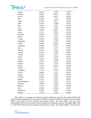
obtained 3,1973 MJ/m2.This result have been obtained from Isparta location. So the worst result have been
obtained from Isparta location by using Nu-SVR method. The lowest RMSE value have been calculated as
0,5266 MJ/m2. The related value is belong to Kars location. So that, the best result have been obtained Kars
location.
Figure 2 : GSR variation of Kars location monthly.
Figure 2 shows 2002 year GSR variation of Kars location monthly. When we examine the variation,
we can observed that estimated value and actual value is very close to each other. The first, fifth, ninth,
tenth month's value are more compatible. It has been observed. We cannot say the same for the third and
sixth month.
As a result, estimating was practiced by using 53 many locations. ELM, SVR, KNN, LR and NU-
SVR methods were used to estimate GSR. Month, altitude, latitude, longitude, vapour pressure deficit and
land surface temperature were used to train networks of methods, as input parameters. These obtained
results have been evaluated statistically. The best result have been obtained by using Nu-SVR method. On
the other hand, the worst result have been obtained by using LR method. Also the other methods gave
compatible results. If researcher study estimating of GSR we may offer them to use ELM, SVR, KNN, and
NU-SVR methods.
REFERENCES
[1] Yuehua L., Yingni J. and Xinxiao C. (2011). Evaluation of three models for calculating daily
global solar radiation at Yushu, in Tibet Int. Conf. Cons. Electronic. Comm. and Network, 1252-
1255.
[2] Al Riza D. F., Gilani S. I. H. and Aris M. S. (2011). Hourly solar radiation estimation using
ambient temperature and relative humidity data Int. J. Environ. Sci. Dev., pp. 188-193.
[3] Park D. C., El-Sharkawi M. A. and Mark II R. J. (1991). Electric load forecasting using artificial
neural network, IEEE Trans. Power Syst.99, pp. 442-449.
[4] Al-Alawi S. M. and Al-Hinai H. A. (1998). An ANN based approach for predicting global solar
radiation in locations with no direct measurement instrumentation, Renew. Energy14 , pp. 199-
204.
[5] Mellit A. and Kalogirou S. A. (2008). Artificial intelligence techniques for photovoltaic
applications: a review Prog. Energy Combust. Sci.34 (5), pp. 574–632.
0
5
10
15
20
25
1 2 3 4 5 6 7 8 9 10 11 12
KARS
Actual value (MJ/m^2 ) Nu-svr value (MJ/m^2)](https://image.slidesharecdn.com/estimationofglobalsolarradiationbyusingmachinelearningmethods-170612081118/85/Estimation-of-global-solar-radiation-by-using-machine-learning-methods-9-320.jpg)
![International Journal of Thales Engineering Sciences (JTHES)
16 | P a g e
www.thalespublisher.com
[6] Şahin M., Yıldız Y., Şenkal O. and Peştamalci V. (2013). Estimation of the vapour pressure deficit
using NOAA-AVHRR data J. of Rem. Sen. 34, pp. 2714-2729.
[7] Şahin M. (2013). Weather Satellites and Remote Sensing LAP LAMBERT Ac. Pub. ISBN: 978-
3-659-33947-9, pp. 1-68.
[8] Becker F. (1987). The Impact of Spectral Emissivity on the Measurement of Land Surface
Temperature International Journal of Remote Sensing 8, pp. 1509–1522.
[9] Altman N. S. (1992). An introduction to kernel and nearest-neighbour nonparametric
regression The American Statistician 46 (3), pp. 175–185.
[10] Smola M., Smola A. J., Ratsch G, Schoölkopf B., Kohlmorgen J. and Vapnik V. (1997).
Predicting time series with support vector machines Proceedings of ICANN’97Springer
LNCS 1327, pp. 999–1004.
[11] Smola A. and Schoölkopf B. (1998). A tutorial on support vector regression. NeuroCOLT
Tech. Rep.TR 1998–030 (Royal Holloway College, London, U.K.)
[12] Soh Y C., Huang G-B. and Lan Y. (2010). Constructive hidden nodes selection of extreme
learning machine for regression Neurocomputing 73, pp. 3191-3199.
[13] Qin A. K., Sugnthan P. N., Huang G.-B. and Zhu Q-Y. (2005). Evolutionary extreme learning
machine The journal of the pattern recognition 38, pp. 1759-1763.
[14] Wang D. H. and Lan Yand Huang G.-B. (2011). Extreme Learning Machines: a survey
Int.J.Mach.Learn&Cyber2, pp. 107-122.
[15] Montgomery D. C. and Peck E. A. (1992). Introduction to linear regression analysis 2nd ed.
Wiley. New York.
[16] Sharif M. and Burn D. H. (2006). Simulating climate change scenarios using an improved K-
nearest neighbor model Journal of Hydrology 325 1-4, pp. 179-196.
[17] Yakowitz S. (1987). Nearest neighbors method for time series analysis Journal of Time
Series Analysis 8, pp. 235-247.
[18] Liang H. and Xi-Long C. (2010). A nu-support vector regression based system for grid
resource monitoring and prediction Acta Automatica Sinica 36, pp. 139–146.
[19] Laurent H., Jobard I. and Toma A. (1998). Validation of satellite and ground-based estimates
of precipitation over the Sahel Atmospheric Research, 47-48, 651-670.
[20] Kendall M. A. and Stuart A. (1963). The advanced theory of statistics Griffin (Ed.), London, p.
1730.
[21] Katiyar K., Kumar A., Pandey C. K. and Das B. (2010). Acomparative study of monthly
mean daily clear sky radiation over India International Journal of Energy and Environment 1,
pp. 177–182.](https://image.slidesharecdn.com/estimationofglobalsolarradiationbyusingmachinelearningmethods-170612081118/85/Estimation-of-global-solar-radiation-by-using-machine-learning-methods-10-320.jpg)