The document describes a study that uses particle swarm optimization to enhance the radiation pattern of a phase array antenna by minimizing sidelobe levels. It first provides background on issues with high sidelobes in phase array antennas, such as power losses and interference. It then summarizes previous research using techniques like genetic algorithms for antenna array optimization. The study models the radiation pattern of linear arrays with different element numbers and calculates gain, finding that gain increases with more elements. However, sidelobe levels also increase relatively. Therefore, the study proposes using particle swarm optimization to optimize current excitation and control sidelobe levels while maintaining a narrow beamwidth.

1. IOSR Journal of Electronics and Communication Engineering (IOSR-JECE)
e-ISSN: 2278-2834,p- ISSN: 2278-8735.Volume 10, Issue 1, Ver. 1 (Jan - Feb. 2015), PP 60-69
www.iosrjournals.org
DOI: 10.9790/2834-10116069 www.iosrjournals.org 60 | Page
Enhancing the Radiation Pattern of Phase Array Antenna Using
Particle Swarm Optimization
1
J.J. Biebuma, 2
B. O. Omijeh, 3
E. L. Jackson
1,2,3
Department of Electronic & Computer Engineering University of Port Harcourt, Rivers State, Nigeria.
Abstract: Phase array antenna radiates a signal pattern whose side lobes compared to the main lobe is higher
than the acceptable value and become more pronounced when the array is steerable (scanning array). Despite
efforts made by array designers to control this defect, have still not solved the problem of power losses in
undesired directions and radio signal interference with other frequency signals. In this paper, a modified
particle swarm optimization program has been proposed. The program finds the values of current excitation
that will minimize sidelobe level and achieve a radiation pattern that matches closely with the desired pattern.
The Particle Swarm Optimization program forms a part of a 24 array antenna model, and the whole idea is
simulated in MATLAB environment. Results obtained are very satisfactory. When fully implemented by array
designers, power losses will greatly reduce and radio link communication will greatly improve.
Keywords: Radiation, Antenna, Optimization, Swarm, Matlab
I. Introduction
One of the setbacks of phase array antenna is power losses due to high sidelobes in its radiation pattern.
Sidelobes map out the portion of the transmitted power that is wasted in undesired direction. Several authors
have carried out research studies on array pattern optimization. Linear antenna array was optimized using
genetic algorithm for reduction in side lobe levels and directivity improvement (Pallavi, 2013). In his paper,
Genetic algorithm Solver in Optimization toolbox of MATLAB was used to obtain maximum reduction in side
lobe level relative to the main beam on both sides of 0° to improve the directivity. Genetic algorithm is an
intellectual algorithm that searches for the optimum element weight of the array antenna. His paper
demonstrated the different ways to apply Genetic algorithm by varying number of elements to optimize the
array pattern. Adaptive feasible mutation with single point crossover showed the performance improvement by
reducing the side lobe level below -10dB in most of the cases and also improved the directivity. The best result
of -21.05dB sidelobe is obtained for 20 elements in 50 generation of GA with best fitness value of 27.2451 and
mean fitness value of 27.3439 and improved the directivity to 16.960
level. The best result of 17.980
directivity
was obtained for 24 elements.
When antennas elements are arrayed in a certain geometrical configuration, the signal induced on them
are combined to form the array output. A plot of the array response as a function of angle is normally referred to
as the array pattern or beam pattern. Synthesizing the array pattern of antenna array has been a subject of several
studies and investigations. The trade-off between the side-lobe levels (SLL) and the half-power beamwidth
(HPBW) stimulate the question answered primarily by Dolph of obtaining the narrowest possible beamwidth for
a given side-lobe level or the smallest side-lobe level for a given beamwidth (Haupt, 1986). This was possible
by using the orthogonal functions of Chebyshev in order to design an optimum radiation pattern (Drabowitch,
etal 1998). However, for large number of elements this procedure becomes quite cumbersome since it requires
matching the array factor expression with an appropriate Chebyshev function (Balanis, 2005). To over-come
this deficiency, Safaai-Jazi proposed a new formulation for the design of Chebyshev arrays based on solving a
system of linear equations (Safaai-Jazi, 1994). The forgoing mentioned investigations either require analytical
formulae or evaluating the gradient of some objective function, which sometimes become formidable to
evaluate. As alternatives, neural network and evolutionary algorithms techniques were used in order to reduce
the side lobes of linear arrays (Dahab, etal 1998). Genetic algorithms (GA) and particle swarm optimization are
well-known evolutionary algorithm techniques (Rahmat-Samii, etal 1999). In GA, a sample of possible
solutions is assumed then mutation, crossover, and selection are employed based on the concept of survival of
the fittest. On the other hand, PSO is a much easier algorithm in which each possible solution is represented as a
particle in the swarm with a certain position and velocity vector. The position and velocity of each particle are
updated according to some fitness function. Some studies have been devoted to compare between the GA and
PSO and a general conclusion has been reached that the PSO shows better performance due to its greater
implementation simplicity and minor computational time.
Since it has been introduced by Kennedy and Eberhard, the PSO is being applied to many fields of endeavor.
Surprisingly, it has been applied to the design of low dispersion fiber Bragg gratings (Basker, etal,
2005), and to the design of corrugated horn antenna.

2. Enhancing the radiation pattern of phase array antenna using particle swarm optimization
DOI: 10.9790/2834-10116069 www.iosrjournals.org 61 | Page
Phased arrays operate using an electrically or mechanically steered beam. Multiple antenna elements
are used, but their transmitted (or received) signals are phase shifted so as to alter the direction of the antenna’s
broadcast. This apparent steering is caused by constructive interference in the direction of interest and
destructive interference in directions of no interest (Balanis, 2005). The phase shifting can be done by analog or
digital phase shifters. With the analog method, varactor diodes, whose reactance can be changed by a bias
voltage, are used to control phase. In the digital domain, there are a variety of digital phase shifter chips that are
used (http://www.microwaves101.com/encyclopedia/phaseshifters.cfm).
II. Theoretical Background Of Phased Array Antennas
Fig 1.1 Uniform linear array of N element along the z-axis Fig 3.1 Geometry of array element of size 2N
A uniform linear array antenna is one whose elements have equal amplitude and are spaced equally
along one dimension. In figure 1.1, maximum beam occurs for θ0= 900
. If we center array about z=0, and
normalize, the array factor will become
……………………… (2.1)
The radiation pattern of a phase array antenna is
Radiation pattern = Element pattern × array factor
For isotropic sources, the radiation pattern is equal to the array factor.
III. Design Methodology
3.1 Modeling of antenna pattern
The electric field of a linear array of isotropic sources is given by
…. (3.2)
Where electric field at angle , n= element number, d= inter-element spacing, = phase shift
per element, = scan angle, I = current excitation, =wavelength
For a uniformly excited array, I= 1.
Rewriting eqn 3.2 in series expansion form
……...…….... (3.3)
This is a geometric series and can be expressed as
; The far field array intensity pattern is given by
.. …………………… (3.4)
substitution gives

3. Enhancing the radiation pattern of phase array antenna using particle swarm optimization
DOI: 10.9790/2834-10116069 www.iosrjournals.org 62 | Page
But 1-
therefore , ………………………………………. (3.5)
The maximum value occurs at and is N. therefore normalizing gives
………………………………………. (3.6)
And the Gain of the beam pattern is
…………………………… (3.7)
As N tends to infinity this becomes a sinc function.
Equation (3.7) is the derived Gain for a linear phase array isotropic antenna of N- elements. In this
paper, the gain of the array of 4, 8, 16, 20 and 24 elements will be calculated using equation (3.7). Besides
calculation, the gain pattern of these numbers of elements at different angles will also be simulated using
MATLAB software to view the effects of element number on the overall antenna radiation pattern.
All through the calculation, d=0.5 =900
, and respectively.
From equation 3.7,
For N=4
=3.99
G (db) =10 log (3.99 =6db
For N=8;
= 8.074; G (db) = 10 log (8.07) = 9.06db
For N= 16
= =15.01
G (db) = 10 log (15.01) =11.8db
For N=20
= ; G (90) = 18.09; G (db) = 10 log (18.09) =12.6db
For N=24
= ; G (90) = 24.90; G (db) = 10 log (24.90) = 14db

4. Enhancing the radiation pattern of phase array antenna using particle swarm optimization
DOI: 10.9790/2834-10116069 www.iosrjournals.org 63 | Page
From the calculations above, it can be seen that the gain of the 4-element array isotropic antenna has
been enhanced from 6db to 14db by adding more elements to the array. To explain this further, the radiation
pattern of the same number of array elements are simulated in MATLAB to view the increase in gain pattern as
the number of radiating elements is increased (fig 3.2, 3.3, 3.4, 3.5, 3.6).
The radiation pattern shows how far down its sidelobes (undesired direction) are from the gain at the
peak of the mainlobe (desired direction). It will be seen that as the number of elements increase in the array, the
sidelobe levels also increase. This indicates that, as the gain in the desired direction increased, the gain in the
undesired direction also increased relatively. Because of this undesirable sidelobes, further improvement will be
done on the normalized gain pattern by optimizing the current excitation function (while keeping constant the
exponential function), that will control sidelobe levels in the far field of the array.
The normalized field pattern is
……………..……………. (3.8)
This pattern is very useful in analyzing array problems showing important radiation properties
such as Half Power Beamwidth, Sidelobes and directivity, and will be used in the next step to generate the fields
of the individual elements with respect to scan angle.
N=4, d=0.5𝞴
Fig 3.2 Gain as a function of scan angle (radians) Fig 3.3 Gain as a function of scan angle
(radians) for N=8, D=0.5𝞴
Fig 3.4 Gain as a function of scan angle (rad) for N=16, d=0.5𝞴 Fig 3.5 Gain as a function of scan angle
(radians) for N=20, d=0.5𝞴
Fig 3.6 Gain as a function of scan angle (rad) for N=24, d=0.5𝞴
3.3.2 Design requirements for particle swamp optimization
In this stage of the work, a 24- element array is being optimized. For uniform excitation, the beamwidth
of such an array is approximately 6° to 7° and sidelobe level about –18 dB. The design goal is that the phased

5. Enhancing the radiation pattern of phase array antenna using particle swarm optimization
DOI: 10.9790/2834-10116069 www.iosrjournals.org 64 | Page
array will have SLL less than –20 dB and beamwidth of approximately 7°. These values are not chosen anyhow
but are based on reference values. For a 24 element array, the lowest SLL level achievable by excitation
optimization is about –20 dB. And by minimizing SLL, the beamwidth cannot be lowered more than 7°.
However, a phased array for any arbitrary SLL and beamwidth can be designed using the same procedure used
here by increasing or decreasing the number of array elements. So, the normalized desired pattern for a 24-
element array is defined as:
The radiation of the array for uniform excitation (an= 1) does not satisfy this design requirements. So,
optimization is necessary. The fitness function (cost function) is defined as the sum of the squares of the excess
far field magnitude above the desired pattern. So,
This type of fitness function definition is widely used for antenna array synthesis problems because it
cuts off sidelobe levels above the desired envelope, while sidelobes below the specifications are neither
penalized nor rewarded. The goal of the optimization process is to find the values of , so that the fitness
function is minimized and the achieved radiation pattern matches closely with the desired pattern.
3.3.3 Particle Swarm Optimization Algorithm And Flowchart
The flowchart for PSO is given in Figure 3.7. The main steps of the PSO algorithm are given as follows:
Step 1: Initialize the particles Xi with initial random positions in search space, and the velocities of particles Vi
in a given range randomly and define these as the best known positions (Pbest) of each particle.
Step 2: Define the objective function f that needs to be optimized.
Step 3: For each particle calculate the distance to the optimal solution called fitness, and apply equation (3.9):
If ………………………………….. 3.9
Step 4: Select globalbest among the Pbest
Step 5: If f(globalbest) reaches to the optimal solution, terminate the algorithm. Otherwise; update the velocity Vi
and the particles Xi according to given equations:
………….. 3.10
…………………………………………….. 3.11
Step 6: Go to Step 3, if stopping criteria are not satisfied
3.3.4 Modified Particle Swarm Optimization
In standard PSO, the velocity at each iteration step is calculated from:
(3.9)
Where r1and r2 are two random numbers between 0 and 1, c1and c2 are acceleration constants, w is the
inertial weight, xpb,n is the coordinate of the personal best position of the particle in nth dimension and xgb,n is the
coordinate of the global best position of the swarm in the nth dimension. The value of both acceleration
constants c1and c2 are taken to be 3, which are commonly used values. The two random variables are used to
simulate the slight unpredictable component of natural swarms. The inertial weight, w, determines to what
extent the particle remains along its original course and is not affected by the pull of personal best and global
best. If tmax is the maximum number of iterations, then, w is expressed as:
W (t) = ……………………………………….…….(3.10)
The modified Gaussian linear equation is:

6. Enhancing the radiation pattern of phase array antenna using particle swarm optimization
DOI: 10.9790/2834-10116069 www.iosrjournals.org 65 | Page
Where, y is a constant whose value is taken to be 1.2. The function has the same initial and final values
as the linear function, but it is characterized by a sharper rate of decrease. A small value of w encourages local
exploitation whereas a larger value of w encourages global exploration. So, it is expected that the sharper fall of
w will increase the rate of convergence without sufficiently reducing global search.
Fig 3.7 Flowchart of Particle Swarm Optimization
Using a simple linear relationship between the variables, the velocity update equation can be modified. This
modified equation can be expressed as:
………. (3.13)
The modified PSO used here consists of this modified velocity update equation along with modified inertial
weight variation function given by (3.11)
The optimization problem is modeled into minimum-maximum problem
IV. Results
4.1 Enhanced Pattern With Respect To Optimized Current Excitation
The results for the main lobe and the first sidelobe peaks of the normalized radiation pattern for 4, 8,
16, 20, and 24 isotropic elements with uniform current excitation are presented in table 4.1. The results for the
optimized current excitations are presented in the Table 4.2, Table 4.3, Table 4.4, table 4.5 and table 4.6 for 4, 8,
16, 20 and 24 elements of the antenna array respectively. For each array, to show that the modified PSO has
suppressed the sidelobe levels much more than the standard PSO, sidelobe levels are given at the end of the
table. The excitation obtained through the algorithms are substituted for I in eqn 3.2 and used in the calculation
of the field pattern for each array. The electric fields for 24 elements are presented in tables 4.7, 4.8, 4.9 and
4.10. Ed are the normalized electric fields of 24 elements with uniform currents, Ed0 are the logarithmic
electric fields elements with uniform currents (I=1), Ed1 are the electric fields with optimized currents and Ed2
are the electric fields with Modified optimized current amplitudes respectively. The radiation patterns for each
set of elements are shown in the figures- fig4.1, Fig. 4.2, Fig. 4.3, fig. 4.4, and fig.4.5(a, b) respectively. Fig 4.6
is plotted from table 4.6. These optimized plots show the smooth reduction in the side lobe level in each case
and meet the objective function of the algorithm of -20db.

7. Enhancing the radiation pattern of phase array antenna using particle swarm optimization
DOI: 10.9790/2834-10116069 www.iosrjournals.org 66 | Page
Table 4.1 Gain and SLL of 4, 8, 16, 20 and 24 element Table 4.2 synthesized currents
with 4 elements
Number of
elements
4 8 16 20 24
Gain 4.79 7.79 9.56 9.999 10.33
Sidelobe
level
-2 -1 2.5 2.6 4.9
Table 4.4 synthesized currents with 16 elements
Table 4.3 synthesized currents with 8 elements
Element
excitation
Uniform
excitation
Standard
Particle
Swamp
Optimization
Modified
Particle
Swamp
Optimization
1 0.7077 0.7843
1 0.5390 0.6000
1 0.3805 0.4078
1 0.2601 0.2471
SLL -18db -20db -23db
HPBW
Table 4.5: Synthesized currents with 20 elements Table 4.6: synthesized currents with 24 elements
Element
excitation
Uniform
excitation
Standard
Particle
Swamp
Optimization
Modified
Particle
Swamp
Optimization
1 0.9493 0.9098
1 0.9386 0.8667
1 0.8671 0.7608
1 0.8177 0.6667
1 0.6832 0.5333
1 0.6334 0.5132
1 0.5094 0.4431
1 0.3933 0.3020
1 0.3021 0.2196
1 0.2997 0.1725
SLL -15db -22db -26db
HPBW
Element
excitation
Uniform
excitation
Standard
Particle Swamp
Optimization
Modified
Particle Swamp
Optimization
1 0.9792 1.0000
1 0.8975 0.9216
SLL -15db -100db -100db
HPBW
Element
excitation
Uniform
excitation
Standard
Particle
Swamp
Optimization
Modified
Particle
Swamp
Optimization
1 0.1452 0.1255
1 0.9228 0.0588
1 0.9323 0.9792
1 0.8646 0.8965
1 0.6184 0.7076
1 0.4226 0.3816
1 0.2636 0.2551
1 0.2636 0.2551
SLL -15db -21db -24db
HPBW
Element
excitation
Uniform
excitation
SPSO MPSO
1 0.0000 0.0000
1 0.1362 0.0311
1 0.2698 0.0655
1 0.3984 0.0982
1 0.5196 0.1313
1 0.6311 0.1539
1 0.7107 0.1967
1 0.8170 0.2284
1 0.8848 0.2643
1 0.9448 0.2953
1 0.9724 0.3964
1 0.9999 0.3811
SLL -15db -21db -25db
HPBW

8. Enhancing the radiation pattern of phase array antenna using particle swarm optimization
DOI: 10.9790/2834-10116069 www.iosrjournals.org 67 | Page
Table 4.7 Generated Electric fields (ed) Table 4.8: Generated Electric fields (ED0)
FIELDS FOR UNIFORMLY EXCITATION CURRENTS
(NORMALIZED)
0.0000 0.0000 0.0000 0.0000 0.0000 0.0001 0.0001
0.0001 0.0002 0.0002 0.0002 0.0003 0.0003 0.0004
0.0005 0.0005 0.0006 0.0007 0.0008 0.0009 0.0010
0.0011 0.0012 0.0013 0.0014 0.0015 0.0016 0.0017
0.0019 0.0020 0.0022 0.0023 0.0024 0.0026 0.0028
0.0029 0.0031 0.0033 0.0034 0.0036 0.0038 0.0040
0.0042 0.0044 0.0046 0.0048 0.0050 0.0053 0.0055
Table 4.9 generated electric fields (ed1) Table 4.10 Generated Electric fields (ED2)
fields for non-uniformly excitation currents
-322.4763 -133.2510 -121.2098 -114.1661 -109.1686 -
105.2922 -102.1250
-99.4472 -97.1275 -95.0815 -93.2512 -91.5956 -
90.0841 -88.6937
-87.4064 -86.2080 -85.0870 -84.0340 -83.0412 -
82.1022 -81.2113
-80.3640 -79.5561 -78.7842 -78.0452 -77.3364 -
76.6554 -76.0002
-75.3689 -74.7598 -74.1715 -73.6024 -73.0516 -
72.5177 -71.9999
-71.4972 -71.0087 -70.5337 -70.0715 -69.6213 -
69.1827 -68.755
-68.3378 -67.9305 -67.5327 -67.1439 -66.7639 -
66.3922 -66.0284
Fig 4.1: radiation pattern of a 4-element array scanned at broadside Fig 4.2 radiation pattern of an 8-element
array scanned at broadside
Fields For Uniformly Excitation Currents (Logarithmic)
-324.2604 -112.4231 -100.3819 -93.3383 -88.3407 -84.4644 -
81.2971
-78.6193 -76.2997 -74.2536 -72.4234 -70.7677 -69.2563 -67.8659
-66.5786 -65.3802 -64.2592 -63.2062 -62.2134 -61.2744 -60.3835
-59.5362 -58.7284 -57.9565 -57.2175 -56.5087 -55.8278 -55.1727
-54.5414 -53.9324 -53.3441 -52.7751 -52.2243 -51.6906 -51.1728
-50.6702 -50.1818 -49.7070 -49.2448 -48.7949 -48.3564 -47.9289
-47.5118 -47.1047 -46.7071 -46.3185 -45.9387 -45.5672 -45.2037
Fields For Non-Uniformly Excitation Currents
-326.8780 -131.7858 -119.7446 -112.7010 -107.7035 -
103.8271 -100.6599
-97.9820 -95.6624 -93.6163 -91.7861 -90.1305 -88.6190
-87.2286
-85.9413 -84.7429 -83.6219 -82.5689 -81.5761 -80.6370
-79.7462
-78.8989 -78.0910 -77.3191 -76.5801 -75.8713 -75.1904
-74.5352
-73.9039 -73.2948 -72.7065 -72.1375 -71.5866 -71.0528
-70.5350
-70.0323 -69.5439 -69.0689 -68.6067 -68.1566 -67.7180
-67.2904
-66.8732 -66.4660 -66.0682 -65.6796 -65.2996 -64.9279
-64.5643

9. Enhancing the radiation pattern of phase array antenna using particle swarm optimization
DOI: 10.9790/2834-10116069 www.iosrjournals.org 68 | Page
Fig 4.3 radiation pattern of a 16-element array scanned at broadside Fig 4.4 radiation pattern of a 20-element
array scanned at broadside
4.5(a) Normalized radiation pattern of a 24 element linear broadside array
Fig 4.5(b) Logarithmic pattern of a 24-element array scanned at broadside Fig 4.6 Normalized weight
against array elements for PSO and MPSO
V. Conclusion
In this paper, the sidelobe level of 4, 8, 16, 20, and 24 isotropic elements have been suppressed using
Particle Swarm Optimization. The Modified Particle Swamp Optimization produces better results than the
Standard Particle Swamp Optimization. The side lobe level decreased up to -25 dB down the main lobe which
represents the high reduction in the side-lobe level which is very much desirable to avoid radio frequency
interference and sidelobe clutters in wireless communications. The side lobe reduction is more useful in GSM

10. Enhancing the radiation pattern of phase array antenna using particle swarm optimization
DOI: 10.9790/2834-10116069 www.iosrjournals.org 69 | Page
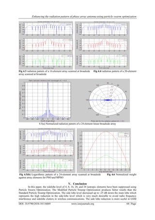
(Global System for Mobile communication), RADAR (Radio Detection And Ranging), SONAR (Sound
Navigation And Ranging) and image mapping; especially in RADAR application where high side lobes can
detect false target and lead to unintended signal jamming.
References
[1]. Balanis. C. A, Antenna Theory: Analysis and Design, 3rd ed., Hoboken: John Wiley, 2005, pp. 300-304.
[2]. Basker S, Alphones A, Suganthan P. N, Genetic Algorithm based design of a reconfigurable antenna array with descrete phase
shifters, Wiley Online library, 2005.
[3]. Dahab.A ,1994: A new technique for linear antenna array processing for reduced sidelobes using neural networks,
[4]. Drabowitch S, Papiernik A, Griffiths H, Encinas J, & Bradford L. Smith, Modern Antennas, Chapman & Hall, London, pp. 400-
402, 1998.
[5]. Haupt R. L, “Directional Antenna System Having Sidelobe Suppression”, Us Patent 4, pp571- 594 Feb 18, 1986.
[6]. Pallavi Joshi, Optimization of linear antenna array using genetic algorithm for reduction in side lobe levels and to improve
directivity, international journal of latest trends in engineering and technology, vol 2, may 2013.
[7]. P-N Designs Inc. (2008, June). Phase Shifters. microwaves101.com [Online]. Available:
http://www.microwaves101.com/encyclopedia/phaseshifters.cfm
[8]. Rahmat-sammii, Y, Colburn, J. S Patch antennas on externally perforated high dielectric constant substrates, 1999, Los Angeles.
[9]. Safaai-Jazi A, A new formulation for the design of Chebychev arrays, IEEE transactions on 42(3), 439-443, 1994
Authors’ Biography
Biebuma Joel Jeremiah holds a B.Eng & M.Sc (S.C.T, Sussex, England) in Electronic & Communication
Engineering, & Ph.D (S.C.U, California, U.S.A) in Telecommunication Engineering . He is a member, Nigeria
Association for Teachers of Technology (MNATT), Member Institute of Electronics and Electrical Engineers
(MIEEE) and Member, Nigeria Society of Engineers. His research interest is in Electronics, Telecommunication,
Antennas, Microwaves etc. He is a prolific writer with numerous technical papers and engineering text books. He is
currently a Senior Lecturer and Ag. HOD, Department of Electronic and Computer Engineering, University of Port
Harcourt, Port Harcourt, Nigeria. He is happily married with Children.
Bourdillon .O. Omijeh holds a B.Eng degree in Electrical/Electronic Engineering, M.Eng and Ph.D .Degrees in
Electronics/Telecommunications Engineering from the University of Port Harcourt & Ambrose Alli University
(A.A.U), Ekpoma respectively. His research areas include: Artificial Intelligence, Robotics, Embedded Systems
Design, Modeling and Simulation of Dynamic systems, Intelligent Metering Systems, Automated Controls,
Telecommunications and ICT. He has over thirty (30) technical papers & publications in reputable International
learned Journals and also, has developed over ten (10) application Software. He is a member, Institute of Electronics
and Electrical Engineers (MIEEE), Member, Nigeria Society of Engineers; and also, a Registered Engineer (COREN).
He is currently a Senior Lecturer & pioneer HOD, Department of Electronic and Computer Engineering, University
of Port Harcourt, Nigeria; and also, a consultant to companies & Institutions. He is happily married with Children.
E-mail: bourdillon.omijeh@uniport.edu.ng.
Jackson Eno Linus holds a B.Eng Degree in Electrical/Electronic Engineering from the University of Uyo, Uyo. Her
research areas includes: voltage regulators, fibre optics, automated controls and antennas. She is currently carrying out
a research work on enhancing the gain of phased array antenna in her Masters’ Degree Programme at Department of
Electronic & Computer Engineering, University of Port Harcourt, Nigeria.