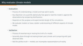
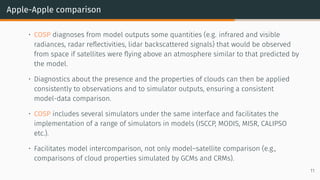
The document discusses model evaluation and validation. It introduces key concepts like evaluation, validation, and the apple-orange problem when directly comparing models and observations. It describes using a satellite simulator like COSP to facilitate apple-to-apple comparisons by simulating what satellites would observe from the model. The document also notes issues with observations like errors and uncertainties that must be considered during evaluation.

1. ASL761 - Class Presentation
Understanding Model Evaluation and Validation
Puneet Sharma
15 October, 2019
Centre for Atmospheric Sciences, IITD

2. Table of contents
1. Introduction
2. Evaluation using observations
3. Next step: Identifying model errors
4. Model-Observations comparison — Apple-Orange problem
5. Conclusion
1

3. Introduction

4. Why evaluate climate models
https://news.ucar.edu/sites/default/files/news/2011/predictFlow2.jpg
2

5. Why evaluate climate models
• Evaluation
– Process of understanding a model and how well it works.
– Key objective is to quantify statistically how good or bad the model is against the
observations by comparing distributions.
– Depends on the purpose and experimental design of the simulations.
– We evaluate models to have a better understanding of different aspects of climate
model.
• Validation
– Process of ascertaining or testing the truth of a model.
– Generally done through recreating known past climate and comparing with past
observed data.
– Not the perfect truth — models are incomplete representations of reality.
3

6. Evaluation using observations

7. Issues with observations
• Observations are not absolute truth.
• Observations can have missing/inaccurate information — depends on
– Duration of records.
– Errors arising due to
* Systematic error — Calibration and instrument issues thus leads to consistent departures from
true value.
* Random error — Unpredictable disturbances thus leads to outliers in the observations.
– Erroneous retrieval algorithms.
– Artifacts in satellite retrievals.
4

8. Issues with observations
Sparse Distribution
90 95 100 105 110
Value
0
5
10
15
20
25
ObservationNumber Sparse Probability Distribution
90 95 100 105 110
Value
0.0
0.1
0.2
0.3
0.4
0.5
Probability
Well Sampled Distribution
90 95 100 105 110
Value
0
1000
2000
3000
ObservationNumber
Probability Distribution
90 95 100 105 110
Value
0.00
0.05
0.10
0.15
0.20
Probability
(a) (b)
(c) (d)
Fig. 9.1 Sampled distributions. Points representing individual observations are randomly sampled
from a distribution with a mean of 100 and a standard deviation of 2. a Sample with 25 points.
b The probability distribution function (PDF) of these points. c Same distribution with a sample of
3000 points. d The PDF of these points
164 9 Model Evaluation
5
Andrew Gettelman (2016) :
Demystifying Climate Models: A Users
Guide to Earth System Models

9. Uncertainty in observations
• Evaluation of climate models also depends on how well do we understand the uncertainty in
observations.
intervals using daily values in the time
series. Generally, positive sensitivities
indicate that N increases with τa, an
indicator of the first aerosol indirect
effect. We note at this point that there
may be limitations to this metric, which
are further discussed in section 3.4.
Figure 6a shows ΔlnN/Δlnτa in SAF
during the entire analysis period and
separately for each season (see the
supporting information for numerical
values and the number of daily samples
used to compute each sensitivity). For
the entire period (“ALL” in Figure 6), the
sensitivity calculated using observations
−0.4
−0.2
0.0
0.2
0.4
0.6
ALL SON DJF MAM JJA
Δln(N)/Δln(τa)Journal of Geophysical Research: Atmospheres 10.1002/2014JD021722
6
Ban-Weiss et al. (2014) :
Evaluating clouds, aerosols, and their
interactions in three global climate
models using satellite simulators and
observations

10. Issues with observations
Understanding the uncertainty in the observations, including
the retrieval algorithms that are used for observations, and
the difference between what the observations and the
model represent is critical for evaluation.
7

11. Next step: Identifying model
errors

12. Identifying model errors
• Majority of errors in model come from the modeled physics — parameterized
processes.
• Model errors (model uncertainty) can arise due to reasons such as
– Internal variability
– Simplistic model physics
– Errors in land-sea coupling in the model.
– Compensating errors
• Once the source of model error pertaining to a specific process is known, the next
step is model improvement.
8

13. Model-Observations comparison
— Apple-Orange problem

14. Conceptualizing satellite simulator
• Large uncertainty persists in simulation of cloud cover and cloud properties (Bony
and Dufresne, 2005).
• Satellites are the first source of global observations.
• Direct comparison between model and observations inconsistent (Apple-Orange
comparison !) since
– Satellite derives the observations through processing radiance values and model
calculates atmospheric variables through prognostic and diagnostic equations.
– The assumptions inherent in the retrieval algorithms of satellite (viewing geometry,
sensors’ sensitivity, vertical overlap of cloud layers etc.) are absent in climate models
• To overcome this problem, satellite simulator was devised
9

15. What is COSP ??
• World Climate Research Programme (WCRP) came up with Cloud Feedback Model
Intercomparison Project (CFMIP) whose objective was to improve the understanding
and evaluation of clouds, cloud feedbacks and changes in regional-scale circulation
and precipitation.
• CFMIP community has developed an integrated satellite simulator, the CFMIP
Observation Simulator Package (COSP) (Bodas-Salcedo et al., 2011).
• COSP is a software tool that enables the simulation of data from several
satelliteborne active and passive sensors from model variables.
• It facilitates the use of satellite data to evaluate models in a consistent way
(Apple-Apple comparison !).
10

16. Apple-Apple comparison
• COSP diagnoses from model outputs some quantities (e.g. infrared and visible
radiances, radar reflectivities, lidar backscattered signals) that would be observed
from space if satellites were flying above an atmosphere similar to that predicted by
the model.
• Diagnostics about the presence and the properties of clouds can then be applied
consistently to observations and to simulator outputs, ensuring a consistent
model-data comparison.
• COSP includes several simulators under the same interface and facilitates the
implementation of a range of simulators in models (ISCCP, MODIS, MISR, CALIPSO
etc.).
• Facilitates model intercomparison, not only model–satellite comparison (e.g.,
comparisons of cloud properties simulated by GCMs and CRMs).
11

17. What is COSP ??
So COSP is basically what satellites would see if they were
inside the climate model !!
12

18. COSP use case
using the MODIS and MISR t distributions from CAM4
and CAM5 (not shown).
fraction, while mid cloud contributes less. Both CAM4
and CAM5 underestimate cloud fraction at all heights,
FIG. 3. Global column-integrated cloud optical depth (t) distributions: (a) MISR, MODIS, and ISCCP from
satellite observations, CAM4, and CAM5, (b) ISCCP from CAM4 and CAM5 at both 0.98 3 1.258 and 1.98 3 2.58
horizontal grid resolutions. Below t5 3.6 there are large intersatellite differences in cloud fraction due to the dif-
ference in detection and treatment of cloud edges and subpixel clouds. Observational agreement below t5 1.3 is
especially poor (see P12, Fig. 4) and is therefore not plotted in (a). CAM t distributions are accumulated over model
columns and include the subgrid-scale variability implied by partly cloudy layers.
AUGUST 2012 K A Y E T A L . 5197
13
Kay et al. (2012) :
Exposing Global Cloud Biases in the
Community Atmosphere Model (CAM)
Using Satellite Observations and Their
Corresponding Instrument Simulators

19. COSP use case
Evolutions of CAM-CESM1
Model
CCSM3
( 2004 )
CCSM3.5
( 2007 )
CCSM4
( Apr 2010 )
CESM1
( Jun 2010 )
Atmosphere CAM3 (L26) CAM3.5 (L26) CAM4 (L26) CAM5 (L30)
Boundary Layer
Turbulence
Holtslag-Boville (93)
Dry Turbulence
Holtslag-Boville Holtslag-Boville
Bretherton-Park (09)
UW Moist Turbulence
Shallow
Convection
Hack (94) Hack Hack
Park-Bretherton (09)
UW Shallow Convection
Deep
Convection
Zhang-McFarlane (95)
Zhang-McFarlane
Neale et al.(08)
Richter-Rasch (08)
Zhang-McFarlane
Neale et al.(08)
Richter-Rasch (08)
Zhang-McFarlane
Neale et al.(08)
Richter-Rasch (08)
Cloud
Macrophysics
Zhang et al. (03)
Zhang et al.
with Park & Vavrus’ mods.
Zhang et al.
with Park & Vavrus’ mods.
Park-Bretherton-Rasch (14)
Revised Cloud Macrophysics
Stratiform
Microphysics
Rasch-Kristjansson (98)
Single Moment
Rasch-Kristian.
Single Moment
Rasch-Kristian.
Single Moment
Morrison and Gettelman (08)
Double Moment
Radiation / Optics CAMRT (01) CAMRT CAMRT
RRTMG
Iacono et al.(08) / Mitchell (08)
Aerosols
Bulk Aerosol Model
(BAM)
BAM BAM
Modal Aerosol Model (MAM)
Liu & Ghan (2009)
Dynamics Spectral Finite Volume (96,04) Finite Volume Finite Volume
Ocean POP2 (L40) POP2.1 (L60) POP2.2 - BGC POP2.2
Land CLM3 CLM3.5 CLM4 - CN CLM4
Sea Ice CSIM4 CSIM4 CICE CICE
http://www.cesm.ucar.edu/events/wg-meetings/2015/presentations/amwg/park2.pdf
14

20. Conclusion

21. Summary
• Evaluation and validation of climate models is important in order to improve the
capabilities of weather forecasting and climate projections.
• Evaluating climate models is a task specific exercise i.e. specific aspects of climate
model are evaluated against specific observations.
• While evaluating the model, the uncertainty, errors and assumptions inherent in
the observations must be taken into account.
• Since a climate model is a stochastic system, it can only be analyzed statistically
and thus requires large number of samples in observations for it’s validation.
15

22. Questions?
15

23. References i
References
Andrew Gettelman, R. B. R.: Demystifying Climate Models, Springer Berlin Heidelberg, URL
https://www.ebook.de/de/product/25136537/andrew_gettelman_richard_b_
rood_demystifying_climate_models.html, 2016.
Ban-Weiss, G. A., Jin, L., Bauer, S. E., Bennartz, R., Liu, X., Zhang, K., Ming, Y., Guo, H., and Jiang, J. H.:
Evaluating clouds, aerosols, and their interactions in three global climate models using satellite
simulators and observations, Journal of Geophysical Research: Atmospheres, 119, 10,876–10,901,
https://doi.org/10.1002/2014JD021722, URL
https://agupubs.onlinelibrary.wiley.com/doi/abs/10.1002/2014JD021722,
2014.

24. References ii
Bodas-Salcedo, A., Webb, M. J., Bony, S., Chepfer, H., Dufresne, J.-L., Klein, S. A., Zhang, Y., Marchand,
R., Haynes, J. M., Pincus, R., and John, V. O.: COSP: Satellite simulation software for model
assessment, Bulletin of the American Meteorological Society, 92, 1023–1043,
https://doi.org/10.1175/2011bams2856.1, 2011.
Bony, S. and Dufresne, J.-L.: Marine boundary layer clouds at the heart of tropical cloud feedback
uncertainties in climate models, Geophysical Research Letters, 32,
https://doi.org/10.1029/2005GL023851, URL
https://agupubs.onlinelibrary.wiley.com/doi/abs/10.1029/2005GL023851,
2005.
Kay, J. E., Hillman, B. R., Klein, S. A., Zhang, Y., Medeiros, B., Pincus, R., Gettelman, A., Eaton, B., Boyle, J.,
Marchand, R., and Ackerman, T. P.: Exposing Global Cloud Biases in the Community Atmosphere
Model (CAM) Using Satellite Observations and Their Corresponding Instrument Simulators,
Journal of Climate, 25, 5190–5207, https://doi.org/10.1175/jcli-d-11-00469.1, 2012.