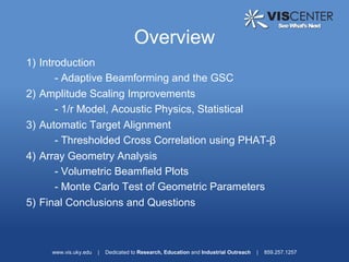
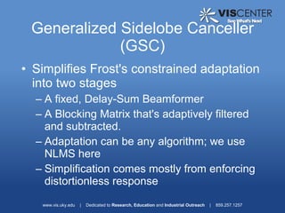
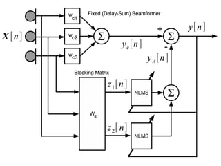
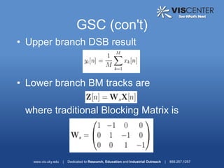
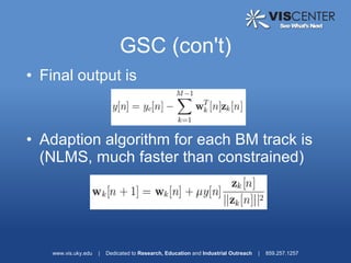
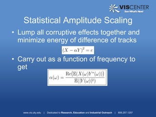
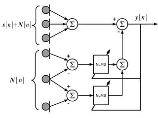
The document discusses enhancements to the generalized sidelobe canceller (GSC) algorithm for audio beamforming. It presents:
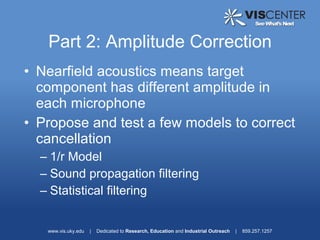
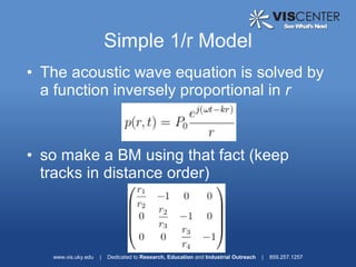
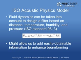
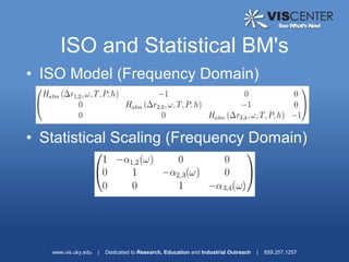
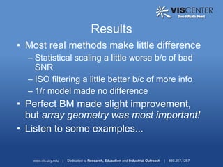
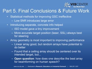
1) Amplitude scaling models to account for near-field effects, including a 1/r model, acoustic physics model, and statistical model. Experimental results found the acoustic physics model provided a small improvement.
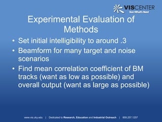
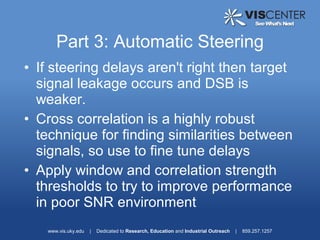
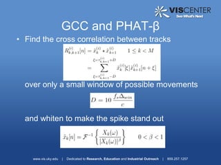
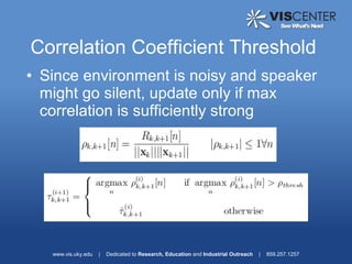
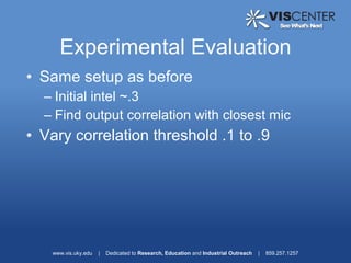
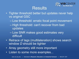
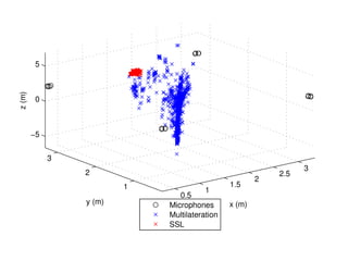
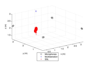
2) Automatic target alignment using cross-correlation and a threshold, but experimental results found this did not improve performance over the standard GSC due to low signal-to-noise ratios.
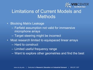
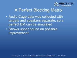
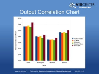
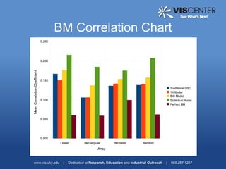
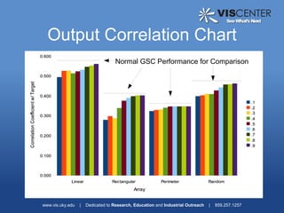
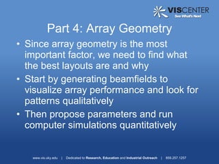
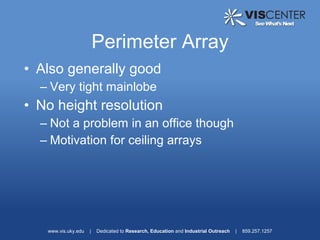
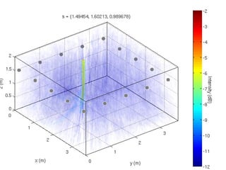
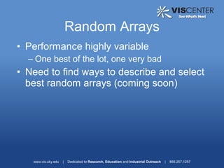
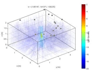
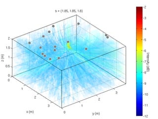
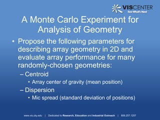
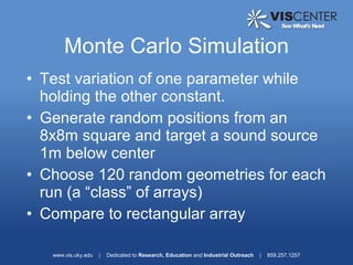
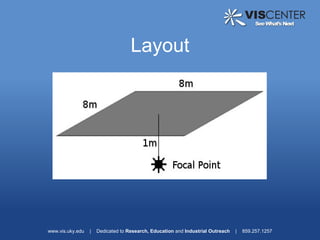
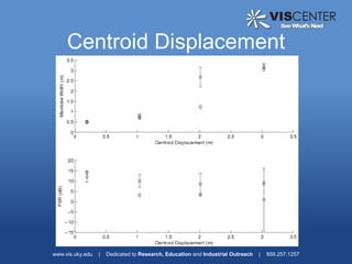
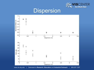
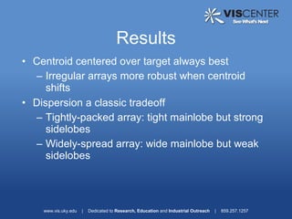
3) Analysis of different array geometries using beamfield plots and simulations, finding array geometry has the largest impact on performance and random arrays have potential if well described.


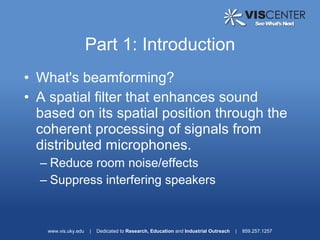
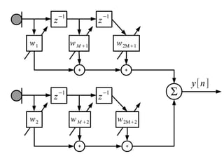
![Adaptive Beamforming
• Optimization of Generalized Filter
Coefficients
T
y[ n]=W [ n] X [n ] opt
– Often requires minimizing output energy
while keeping target component unchanged
• Estimate statistics on the fly
– Input Correlation Matrix unknown/changing
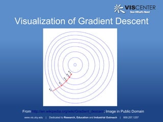
• Gradient Descent Toward Optimal Taps
– Constrained Lowest Energy Output Forms
Unique Minimum to Bowl-Shaped Surface
www.vis.uky.edu | Dedicated to Research, Education and Industrial Outreach | 859.257.1257](https://image.slidesharecdn.com/presentation-12602889112427-phpapp02/85/MSEE-Defense-4-320.jpg)


![Frost Algorithm
• Solution to the constrained optimization
subject to the constraint (C a selection
matrix)
The constraint vector dictates the sum of
column weights, often F = [1 0 0 0...]
• Solution (P and F constant matrices):
www.vis.uky.edu | Dedicated to Research, Education and Industrial Outreach | 859.257.1257](https://image.slidesharecdn.com/presentation-12602889112427-phpapp02/85/MSEE-Defense-51-320.jpg)


![사례로 풀어보는 마케팅 전략[120517]](https://cdn.slidesharecdn.com/ss_thumbnails/120517-120517112704-phpapp01-thumbnail.jpg?width=640&height=640&fit=bounds)
![Ppt2010교육[2011.10.25] (4prt)](https://cdn.slidesharecdn.com/ss_thumbnails/ppt20102011-10-254prt-120515070658-phpapp01-thumbnail.jpg?width=640&height=640&fit=bounds)