Presented in this short document is a description of how to estimate deterministic and stochastic non-parametric finite impulse response (FIR) models in IMPL applied to industrial gas furnace data identical to that found in TSE-GFD-IMF using parametric transfer-functions. The methodology of time-series analysis or system identification involves essentially three (3) stages (Box and Jenkins, 1976): (1) model structure identification, (2) model parameter estimation and (3) model checking and diagnostics. We do not address (1) which requires stationarity and seasonality assessment/adjustment, auto-, cross- and partial-correlation, etc. to establish the parametric transfer function polynomial degrees especially when we are using non-parametric FIR estimation. Instead we focus only on the parameter estimation and diagnostics. These types of parameter estimation problems involve dynamic and nonlinear relationships shown below and we solve these using IMPL’s Sequential Equality-Constrained QP Engine (SECQPE) and Supplemental Observability, Redundancy and Variability Estimator (SORVE). Other types of non-parametric identification known as Subspace Identification (Qin, 2006) and can used to estimate state-space models.

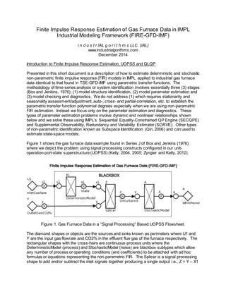
1. Finite Impulse Response Estimation of Gas Furnace Data in IMPL
Industrial Modeling Framework (FIRE-GFD-IMF)
i n d u s t r IAL g o r i t h m s LLC. (IAL)
www.industrialgorithms.com
December 2014
Introduction to Finite Impulse Response Estimation, UOPSS and QLQP
Presented in this short document is a description of how to estimate deterministic and stochastic
non-parametric finite impulse response (FIR) models in IMPL applied to industrial gas furnace
data identical to that found in TSE-GFD-IMF using parametric transfer-functions. The
methodology of time-series analysis or system identification involves essentially three (3) stages
(Box and Jenkins, 1976): (1) model structure identification, (2) model parameter estimation and
(3) model checking and diagnostics. We do not address (1) which requires stationarity and
seasonality assessment/adjustment, auto-, cross- and partial-correlation, etc. to establish the
parametric transfer function polynomial degrees especially when we are using non-parametric
FIR estimation. Instead we focus only on the parameter estimation and diagnostics. These
types of parameter estimation problems involve dynamic and nonlinear relationships shown
below and we solve these using IMPL’s Sequential Equality-Constrained QP Engine (SECQPE)
and Supplemental Observability, Redundancy and Variability Estimator (SORVE). Other types
of non-parametric identification known as Subspace Identification (Qin, 2006) and can used to
estimate state-space models.
Figure 1 shows the gas furnace data example found in Series J of Box and Jenkins (1976)
where we depict the problem using signal processing constructs configured in our unit-
operation-port-state superstructure (UOPSS) (Kelly, 2004, 2005; Zyngier and Kelly, 2012).
Figure 1. Gas Furnace Data in a “Signal Processing” Based UOPSS Flowsheet.
The diamond shapes or objects are the sources and sinks known as perimeters where U1 and
Y are the input gas flowrate and CO2% in the effluent flue gas of the furnace respectively. The
rectangular shapes with the cross-hairs are continuous-process units where the
DeterministicModel (process) and StochasticModel (noise) are blackbox subtypes which allow
any number of process or operating conditions (and coefficients) to be attached with ad hoc
formulas or equations representing the non-parametric FIR. The Splicer is a signal processing
shape to add and/or subtract the inlet signals together producing a single output i.e., Z = Y – X1

2. in our case. The circles with and without cross-hairs are outlet and inlet port-states respectively.
Port-states are unambiguous interfaces between up and downstream unit-operations.
The deterministic FIR model in discrete-time or difference form (versus z-transform or
backwards-shift operator-based quotients of rational polynomials) is defined as follows:
X1,0 = G0*U1,0+G1*U1,1+G2*U1,2+G3*U1,3+G4*U1,4+G5*U1,5+G6*U1,6+G7*U1,7+G8*U1,8+G9*U1,9+G10*U1,10
where U1 is the exogenous input signal minus its mean of -0.057 at time-periods t-1, t-2, …, t-
10 and X1is the “deterministic state” at time-period t-0. The corresponding parameters or
coefficients are G0, G1, …, G10 are the FIR values for each time-shift or lag in the past where
G0 is typically set to zero (0.0) given discrete-time sampling and some of the initial coefficients
G1, etc. will also be effectively zero (0.0) given the dead-time or inherent delay in the system.
The static or steady-state gain of each input with respect to each output can be easily calculated
from the dynamic gains or FIR’s by taking their sum. During the initial part of the estimation
procedure, the number of FIR’s is typically set to some number greater than expected. Then,
using the parameter variances and the Student-t statistics (parameter confidence-intervals) the
actual number is reduced to hopefully avoid over-parameterization which is a well-known
disadvantage of FIR’s and non-parametric models in general.
Similarly, the stochastic FIR model or unmeasured noise disturbance model is also defined as
follows (Schoukens et. al. 2011):
A,0 = H0*Z,0+H1*Z,1+H2*Z,2+H3*Z,3+H4*Z,4+H5*Z,5+H6*Z,6+H7*Z,7+H8*Z,8+H9*Z,9+H10*Z,10
where A is the assumed white-noise input signal and Z is the “stochastic state” which is equal to
Z = Y – X1 and the time-series Y is also minus its mean of 53.51. The parameters H0, H1, …,
H10 and actually represent the “inverse” of stochastic noise model in non-parametric form. The
noise model is essentially a time- or frequency-dependent weighting filter and is very important
to ensure that the A-series is independent and identically distributed (MacGregor and Fogal,
1995; Shreesha and Gudi, 2004; Schoukens et. al. 2011) which is squared, summed and
minimized in the objective function of the prediction error or nonlinear least-squares regression.
Without this noise filter, the estimation is well-understood to be biased yielding inaccurate FIR
coefficients but unfortunately makes the estimator nonlinear since H and Z are variables.
From a quantity-logic-quality phenomena (QLQP) perspective, the time-series U1, Y, Z and A
found in Figure 1 are considered as flows or more appropriately signal-flows or data. However,
in our IML implementation found in Appendix A we collapse the three (3) continuous-processes
into one blackbox model as shown by the dotted-line box in Figure 1 where the flows of U1, Y, Z
and A are now considered as conditions and the G and H parameters are static coefficients in
the IMPL semantics.
Once the FIR parameters are known then these can be straightforwardly implemented into
advanced process controllers such as found in APC-IMF-Julia. It should also be stressed that
for multiple-input, multiple-output (MIMO) processes, the design of the input time-series plays
an important role in the success of regressing good and useful dynamic representations such as
transfer-function, state-space and FIR models where a novel design of the external excitation or
dither signals can be found in DSDP-CLE-IMF for open- and/or closed-loop identification.
Industrial Modeling Framework (IMF), IMPL and SSIIMPLE

3. To implement the mathematical formulation of this and other systems, IAL offers a unique
approach and is incorporated into our Industrial Modeling Programming Language we call IMPL.
IMPL has its own modeling language called IML (short for Industrial Modeling Language) which
is a flat or text-file interface as well as a set of API's which can be called from any computer
programming language such as C, C++, Fortran, C#, VBA, Java (SWIG), Python (CTYPES)
and/or Julia (CCALL) called IPL (short for Industrial Programming Language) to both build the
model and to view the solution. Models can be a mix of linear, mixed-integer and nonlinear
variables and constraints and are solved using a combination of LP, QP, MILP and NLP solvers
such as COINMP, GLPK, LPSOLVE, SCIP, CPLEX, GUROBI, LINDO, XPRESS, CONOPT,
IPOPT, KNITRO and WORHP as well as our own implementation of SLP called SLPQPE
(Successive Linear & Quadratic Programming Engine) which is a very competitive alternative to
the other nonlinear solvers and embeds all available LP and QP solvers.
In addition and specific to DRR problems, we also have a special solver called SECQPE
standing for Sequential Equality-Constrained QP Engine which computes the least-squares
solution and a post-solver called SORVE standing for Supplemental Observability, Redundancy
and Variability Estimator to estimate the usual DRR statistics. SECQPE also includes a
Levenberg-Marquardt regularization method for nonlinear data regression problems and can be
presolved using SLPQPE i.e., SLPQPE warm-starts SECQPE. SORVE is run after the
SECQPE solver and also computes the well-known "maximum-power" gross-error statistics
(measurement and nodal/constraint tests) to help locate outliers, defects and/or faults i.e., mal-
functions in the measurement system and mis-specifications in the logging system.
The underlying system architecture of IMPL is called SSIIMPLE (we hope literally) which is short
for Server, Solvers, Interfacer (IML), Interacter (IPL), Modeler, Presolver Libraries and
Executable. The Server, Solvers, Presolver and Executable are primarily model or problem-
independent whereas the Interfacer, Interacter and Modeler are typically domain-specific i.e.,
model or problem-dependent. Fortunately, for most industrial planning, scheduling,
optimization, control and monitoring problems found in the process industries, IMPL's standard
Interfacer, Interacter and Modeler are well-suited and comprehensive to model the most difficult
of production and process complexities allowing for the formulations of straightforward
coefficient equations, ubiquitous conservation laws, rigorous constitutive relations, empirical
correlative expressions and other necessary side constraints.
User, custom, adhoc or external constraints can be augmented or appended to IMPL when
necessary in several ways. For MILP or logistics problems we offer user-defined constraints
configurable from the IML file or the IPL code where the variables and constraints are
referenced using unit-operation-port-state names and the quantity-logic variable types. It is also
possible to import a foreign *.ILP file (row-based MPS file) which can be generated by any
algebraic modeling language or matrix generator. This file is read just prior to generating the
matrix and before exporting to the LP, QP or MILP solver. For NLP or quality problems we offer
user-defined formula configuration in the IML file and single-value and multi-value function
blocks writable in C, C++ or Fortran. The nonlinear formulas may include intrinsic functions
such as EXP, LN, LOG, SIN, COS, TAN, MIN, MAX, IF, NOT, EQ, NE, LE, LT, GE, GT and CIP,
LIP, SIP and KIP (constant, linear and monotonic spline interpolations) as well as user-written
extrinsic functions (XFCN). It is also possible to import another type of foreign file called the
*.INL file where both linear and nonlinear constraints can be added easily using new or existing
IMPL variables.
Industrial modeling frameworks or IMF's are intended to provide a jump-start to an industrial
project implementation i.e., a pre-project if you will, whereby pre-configured IML files and/or IPL

4. code are available specific to your problem at hand. The IML files and/or IPL code can be
easily enhanced, extended, customized, modified, etc. to meet the diverse needs of your project
and as it evolves over time and use. IMF's also provide graphical user interface prototypes for
drawing the flowsheet as in Figure 1 and typical Gantt charts and trend plots to view the solution
of quantity, logic and quality time-profiles. Current developments use Python 2.3 and 2.7
integrated with open-source Gnome Dia and Matplotlib modules respectively but other
prototypes embedded within Microsoft Excel/VBA for example can be created in a
straightforward manner.
However, the primary purpose of the IMF's is to provide a timely, cost-effective, manageable
and maintainable deployment of IMPL to formulate and optimize complex industrial
manufacturing systems in either off-line or on-line environments. Using IMPL alone would be
somewhat similar (but not as bad) to learning the syntax and semantics of an AML as well as
having to code all of the necessary mathematical representations of the problem including the
details of digitizing your data into time-points and periods, demarcating past, present and future
time-horizons, defining sets, index-sets, compound-sets to traverse the network or topology,
calculating independent and dependent parameters to be used as coefficients and bounds and
finally creating all of the necessary variables and constraints to model the complex details of
logistics (discrete) and quality (nonlinear) industrial optimization problems. Instead, IMF's and
IMPL provide, in our opinion, a more elegant and structured approach to industrial modeling and
solving so that you can capture the benefits of advanced decision-making faster, better and
cheaper.
Finite Impulse Response Estimation of Gas Furnace Data Synopsis
After iterating using SECQPE several times and setting certain G and H coefficients to zero
(0.0) depending on their reported confidence-intervals from SORVE, which is the typical
protocol especially with non-parametric estimation, their values with two (2) times their
standard-error are shown below:
G0 = 0.0
G1 = 0.0
G2 = 0.0
G3 = -0.534 +/- 0.15
G4 = -0.667 +/- 0.16
G5 = -0.861 +/- 0.16
G6 = -0.496 +/- 0.16
G7 = -0.260 +/- 0.13
G8 = -0.123 +/- 0.10
G9 = 0.0
G10 = 0.0
H0 = 1.0
H1 = -1.522 +/- 0.10
H2 = 0.613 +/- 0.10
H5 = 0.0
H6 = 0.0
H7 = 0.0
H8 = 0.0
H9 = 0.0
H10 = 0.0
The objective function value computed is 16.9 in twelve (12) iterations of SECQPE. The
reported standard-error of the residuals is 16.9/296 = 0.0571 which approximates the standard-
deviation of the (hopefully) white-noise residuals of time-series A. The absolute values for H1
and H2 are almost identical to those found in Box and Jenkins (1976) which is consistent with
the fact that they also used an auto-regressive (AR) noise model. In addition, no significant

5. auto-correlation of the residuals (our time-series A) was detected confirming that the estimation
should be unbiased.
The static gain (i.e., the first-order partial derivative of how U1 affects Y) using the truncated
impulse response G is -2.941 +/- 1.02 which is close to the steady-state gain reported in TSE-
GFD-IMF of (-0.53-0.37-0.51)/(1-0.57-0.01) = -3.357 by setting the backwards shift operator (z^-
1) to unity (1.0) where the dead-times are identical to three (3) time-periods. Although there is
over a 10% difference between the two static gain estimates, this is not uncommon when fitting
its value from passive or happenstance data which may include some form of feedback (closed-
loop interactions) as opposed to a well-designed, open/closed-loop PRBS/GBNS input/dither
signal (DSDP-CLE-IMF).
In summary, we have highlighted the application of finite impulse response estimation (FIRE)
using the industrial gas furnace data (Series J) from Box and Jenkins (1976) for both the
deterministic and stochastic terms. The model was formulated in IMPL and solved successfully
using its SECQPE and SORVE and can also be used to estimate static gains of the system
which would be useful in further steady-state process optimization (active) and/or process
monitoring (passive) applications.
References
Box, G.E.P., Jenkins, G.M., “Time-series analysis: forecasting and control”, revised edition,
Holden Day, Oakland, CA, 389-400 and Series J. (1976).
MacGregor, J.F., and Fogal, D.T., “Closed-loop identification: the role of the noise model and
prefilters”, Journal of Process Control, 5, 163, 171, (1995).
Shreesha, C., Gudi, R.D., “Analysis of pre-filter based closed-loop control-relevant identification
methodologies”, Canadian Journal of Chemical Engineering, 82, (2004).
Kelly, J.D., "Production modeling for multimodal operations", Chemical Engineering Progress,
February, 44, (2004).
Kelly, J.D., "The unit-operation-stock superstructure (UOSS) and the quantity-logic-quality
paradigm (QLQP) for production scheduling in the process industries", In: MISTA 2005
Conference Proceedings, 327, (2005).
Qin, J.S., “An overview of subspace identification”, Computers and Chemical Engineering,
1502-1513, (2006).
Kelly, J.D., Zyngier, D., "A new and improved MILP formulation to optimize observability,
redundancy and precision for sensor network problems", American Institute of Chemical
Engineering Journal, 54, 1282, (2008).
Schoukens, J., Rolain, Y., Vandersteen, G., Pintelon, R., “User friendly Box-Jenkins
identification using nonparametric noise models, 50th
IEEE Conference on Decision and Control
European Control Conference (CDC-ECC), Orlando, Florida, USA, December, (2011).
IAL, “Time series estimation of gas furnace data industrial modeling framework (TSE-GFD-
IMF)”, Slideshare, August, 2014.

6. IAL, “Advanced process control (APC) industrial modeling framework in the Julia programming
language (APC-IMF-Julia)”, Slideshare, October, 2014.
IAL, “Dither signal design problem for closed-loop estimation industrial modeling framework
(DSDP-CLE-IMF)”, Slideshare, December, 2014.
Appendix A – FIRE-GFD-IMF.IML File
i M P l (c)
Copyright and Property of i n d u s t r I A L g o r i t h m s LLC.
!!!!!!!!!!!!!!!!!!!!!!!!!!!!!!!!!!!!!!!!!!!!!!!!!!!!!!!!!!!!!!!!!!!!!!!!!!!!!!!!
! Calculation Data (Parameters)
!!!!!!!!!!!!!!!!!!!!!!!!!!!!!!!!!!!!!!!!!!!!!!!!!!!!!!!!!!!!!!!!!!!!!!!!!!!!!!!!
&sCalc,@sValue
START,0.0
BEGIN,7.0
END,296.0
PERIOD,1.0
SE,1.0 !0.0571 != 16.9/296
LRGBND,1d+2
gbnd,1d+2
hbnd,1d+2
&sCalc,@sValue
!!!!!!!!!!!!!!!!!!!!!!!!!!!!!!!!!!!!!!!!!!!!!!!!!!!!!!!!!!!!!!!!!!!!!!!!!!!!!!!!
! Chronological Data (Periods)
!!!!!!!!!!!!!!!!!!!!!!!!!!!!!!!!!!!!!!!!!!!!!!!!!!!!!!!!!!!!!!!!!!!!!!!!!!!!!!!!
@rPastTHD,@rFutureTHD,@rTPD
START,END,PERIOD
@rPastTHD,@rFutureTHD,@rTPD
!!!!!!!!!!!!!!!!!!!!!!!!!!!!!!!!!!!!!!!!!!!!!!!!!!!!!!!!!!!!!!!!!!!!!!!!!!!!!!!!
! Constant Data (Parameters)
!!!!!!!!!!!!!!!!!!!!!!!!!!!!!!!!!!!!!!!!!!!!!!!!!!!!!!!!!!!!!!!!!!!!!!!!!!!!!!!!
&sData,@sValue
u1,-0.052
,0.057
,0.235
,0.396
,0.43
,0.498
,0.518
,0.405
,0.184
,-0.123
,-0.531
,-0.998
,-1.364
,-1.463
,-1.245
,-0.757
,-0.418
,-0.136
,0.145
,0.492
,0.828
,0.923
,0.932
,0.948
,1.044
,1.32
,1.832
,2.033
,1.991
,1.923
,1.889
,1.824
,1.665
,1.322
,0.847
,0.417
,0.172
,0.145
,0.388
,0.702
,1.017
,1.466
,2.727
,2.891
,2.869
,2.54

7. ,1.986
,1.542
,1.271
,1.296
,1.665
,1.962
,2.08
,1.872
,0.592
,0.179
,0.066
,0.221
,0.728
,1.076
,1.203
,1.212
,1.169
,1.178
,1.28
,1.314
,1.214
,0.97
,0.677
,0.312
,-0.223
,-1.023
,-1.494
,-1.742
,-1.768
,-1.399
,-0.887
,-0.513
,-0.374
,-0.52
,-0.903
,-1.559
,-1.818
,-1.834
,-1.689
,-1.417
,-1.144
,-0.87
,-0.467
,0.097
,0.845
,1
,0.987
,1.063
,1.194
,1.255
,1.111
,0.652
,-0.023
,-0.257
,-0.231
,-0.096
,-0.052
,-0.13
,-0.198
,-0.172
,0.05
,0.311
,0.387
,0.159
,-0.366
,-1.082
,-2.218
,-2.537
,-2.659
,-2.453
,-1.733
,-1.289
,-1.024
,-0.853
,-0.819
,-0.828
,-0.743
,-0.487
,-0.359
,-0.214
,0.057
,0.46
,0.898
,1.342
,1.664
,1.803
,1.74
,1.542
,1.05
,0.705
,0.634
,0.634
,0.689
,0.804
,0.957

8. ,1.05
,1.025
,0.847
,0.456
,-0.104
,-0.496
,-0.546
,-0.367
,-0.137
,0.008
,0.117
,0.218
,0.358
,0.574
,0.623
,0.617
,0.63
,0.649
,0.728
,0.99
,1.394
,1.517
,1.41
,0.829
,0.275
,-0.18
,-0.657
,-1.042
,-1.212
,-1.118
,-0.619
,0.09
,0.613
,0.7
,0.541
,0.166
,-0.253
,-0.64
,-0.99
,-1.161
,-1.126
,-0.816
,-0.279
,0.12
,0.141
,0.057
,0.058
,0.266
,0.613
,0.839
,0.915
,0.975
,0.919
,0.473
,-0.279
,-0.902
,-1.756
,-2.321
,-2.442
,-2.416
,-2.273
,-1.996
,-1.682
,-1.204
,-0.512
,-0.08
,0.033
,0.007
,-0.078
,-0.219
,-0.477
,-0.814
,-1.186
,-1.382
,-1.365
,-1.118
,-0.756
,-0.577
,-0.525
,-0.568
,-0.656
,-0.791
,-0.982
,-1.289
,-1.571
,-1.562
,-1.092
,-0.431
,-0.103
,0.05
,-0.035
,-0.563
,-1.029
,-1.468
,-1.801

9. ,-1.972
,-1.967
,-1.904
,-1.895
,-1.737
,-1.245
,-0.973
,-0.861
,-0.741
,-0.81
,-0.99
,-1.066
,-0.819
,-0.338
,0.242
,0.719
,0.766
,0.662
,0.558
,0.66
,1
,1.28
,1.306
,0.881
,0.159
,0.082
,0.439
,0.979
,1.089
,0.923
,0.584
,0.15
,-0.401
,-0.691
,-0.89
,-0.972
,-0.871
,-0.588
,-0.367
,-0.219
,-0.101
,0.024
,0.159
,0.308
,0.337
,0.057
,-0.436
,-0.702
,-0.767
,-0.683
,-0.471
,-0.147
,0.091
,0.261
,0.31
,0.252
,0.188
,0.074
,-0.125
,-0.205
y,0.29
,0.09
,-0.01
,-0.01
,-0.11
,-0.41
,-0.81
,-1.11
,-1.31
,-1.51
,-1.51
,-1.11
,-0.51
,0.49
,1.39
,2.49
,3.29
,3.29
,2.89
,2.19
,1.49
,0.79
,-0.31
,-1.21
,-1.91
,-2.31
,-2.71
,-3.01
,-3.51
,-4.31
,-5.11
,-5.61
,-5.91
,-6.01
,-6.01

10. ,-5.91
,-5.41
,-4.51
,-3.51
,-2.41
,-1.71
,-1.61
,-1.81
,-2.31
,-3.51
,-5.21
,-6.51
,-7.71
,-7.91
,-7.51
,-6.61
,-5.71
,-5.31
,-5.21
,-5.61
,-6.31
,-6.31
,-5.41
,-4.11
,-2.91
,-2.01
,-1.91
,-2.31
,-3.01
,-3.41
,-3.71
,-3.91
,-4.11
,-4.21
,-4.31
,-4.21
,-3.81
,-3.21
,-2.21
,-0.71
,0.89
,2.49
,3.39
,3.99
,3.79
,3.09
,2.49
,1.89
,1.89
,2.89
,3.69
,4.49
,4.89
,4.89
,4.59
,4.19
,3.49
,2.49
,1.19
,-0.31
,-1.41
,-1.91
,-2.51
,-3.01
,-3.11
,-2.51
,-1.71
,-1.11
,-0.51
,-0.11
,0.09
,0.19
,0.29
,0.29
,0.29
,-0.21
,-0.51
,-0.61
,-0.11
,1.09
,2.89
,4.49
,5.89
,6.69
,6.49
,5.89
,4.89
,4.09
,3.39
,2.89
,2.49
,2.19
,1.79
,1.49
,0.89

11. ,0.19
,-0.71
,-1.91
,-2.91
,-4.11
,-4.71
,-5.01
,-4.81
,-4.31
,-3.71
,-3.11
,-2.81
,-2.61
,-2.81
,-3.01
,-3.11
,-3.31
,-3.11
,-2.31
,-1.21
,-0.31
,0.39
,0.59
,0.49
,0.09
,-0.31
,-0.51
,-0.71
,-1.21
,-1.61
,-1.91
,-1.91
,-2.11
,-2.31
,-2.81
,-3.51
,-4.11
,-4.21
,-3.81
,-2.91
,-1.71
,-0.51
,0.49
,1.79
,2.39
,2.39
,1.09
,-0.01
,-1.11
,-1.41
,-1.21
,-0.51
,0.29
,1.09
,1.89
,2.39
,2.39
,1.69
,0.89
,0.19
,0.09
,0.09
,-0.31
,-1.01
,-1.51
,-2.11
,-2.51
,-2.61
,-1.11
,-0.01
,2.09
,4.49
,5.99
,6.49
,6.89
,6.99
,6.69
,6.19
,5.49
,4.09
,2.89
,1.69
,0.99
,0.59
,0.59
,0.89
,1.99
,2.69
,3.49
,3.79
,3.89
,3.49
,2.89
,2.39
,1.99

12. ,1.79
,1.69
,1.89
,2.49
,2.99
,3.59
,3.79
,3.29
,2.09
,1.49
,0.59
,0.79
,1.79
,2.89
,3.69
,4.29
,4.79
,5.09
,5.29
,5.29
,5.09
,4.49
,3.89
,3.49
,2.89
,2.79
,2.89
,2.89
,2.49
,1.69
,0.49
,-0.51
,-1.51
,-1.91
,-1.91
,-2.41
,-3.11
,-3.51
,-3.51
,-1.51
,0.49
,1.59
,0.99
,-0.71
,-2.11
,-2.71
,-2.31
,-1.51
,-0.71
,0.29
,0.99
,1.39
,1.39
,1.29
,0.89
,0.19
,-0.21
,-0.71
,-0.91
,-0.91
,-0.51
,0.79
,2.49
,3.49
,4.49
,5.09
,4.99
,4.79
,4.29
,3.79
,3.49
&sData,@sValue
!!!!!!!!!!!!!!!!!!!!!!!!!!!!!!!!!!!!!!!!!!!!!!!!!!!!!!!!!!!!!!!!!!!!!!!!!!!!!!!!
! Construction Data (Pointers)
!!!!!!!!!!!!!!!!!!!!!!!!!!!!!!!!!!!!!!!!!!!!!!!!!!!!!!!!!!!!!!!!!!!!!!!!!!!!!!!!
&sUnit,&sOperation,@sType,@sSubtype,@sUse
BLACKBOX,,processc,blackbox,,
&sUnit,&sOperation,@sType,@sSubtype,@sUse
!!!!!!!!!!!!!!!!!!!!!!!!!!!!!!!!!!!!!!!!!!!!!!!!!!!!!!!!!!!!!!!!!!!!!!!!!!!!!!!!
! Condition Data (Properties)
!!!!!!!!!!!!!!!!!!!!!!!!!!!!!!!!!!!!!!!!!!!!!!!!!!!!!!!!!!!!!!!!!!!!!!!!!!!!!!!!
&sCondition
Y
U1
X1
Z
A
&sCondition
&sCoefficient,@sType,@sPath_Name,@sLibrary_Name,@sFunction_Name,@iNumber_Conditions,@rPerturb_Size,@sCondition_Names
g0,static

13. g1,static
g2,static
g3,static
g4,static
g5,static
g6,static
g7,static
g8,static
g9,static
g10,static
h0,static
h1,static
h2,static
h3,static
h4,static
h5,static
h6,static
h7,static
h8,static
h9,static
h10,static
&sCoefficient,@sType,@sPath_Name,@sLibrary_Name,@sFunction_Name,@iNumber_Conditions,@rPerturb_Size,@sCondition_Names
&sUnit,&sOperation,&sCondition,@rCondition_Lower,@rCondition_Upper,@rCondition_Target
BLACKBOX,,Y,-LRGBND,LRGBND,
BLACKBOX,,U1,-LRGBND,LRGBND,
BLACKBOX,,X1,-LRGBND,LRGBND,
BLACKBOX,,Z,-LRGBND,LRGBND,
BLACKBOX,,A,-LRGBND,LRGBND,
&sUnit,&sOperation,&sCondition,@rCondition_Lower,@rCondition_Upper,@rCondition_Target
&sUnit,&sOperation,&sCoefficient,@rCoefficient_Lower,@rCoefficient_Upper,@rCoefficient_Target
BLACKBOX,,g0, 0.0,0.0,
BLACKBOX,,g1, -0*gbnd,0*gbnd,
BLACKBOX,,g2, -0*gbnd,0*gbnd,
BLACKBOX,,g3, -gbnd,gbnd,
BLACKBOX,,g4, -gbnd,gbnd,
BLACKBOX,,g5, -gbnd,gbnd,
BLACKBOX,,g6, -gbnd,gbnd,
BLACKBOX,,g7, -gbnd,gbnd,
BLACKBOX,,g8, -gbnd,gbnd,
BLACKBOX,,g9, -0*gbnd,0*gbnd,
BLACKBOX,,g10,-0*gbnd,0*gbnd,
BLACKBOX,,h0, 1.0,1.0,
BLACKBOX,,h1, -hbnd,hbnd,
BLACKBOX,,h2, -hbnd,hbnd,
BLACKBOX,,h3, -0*hbnd,0*hbnd,
BLACKBOX,,h4, -0*hbnd,0*hbnd,
BLACKBOX,,h5, -0*hbnd,0*hbnd,
BLACKBOX,,h6, -0*hbnd,0*hbnd,
BLACKBOX,,h7, -0*hbnd,0*hbnd,
BLACKBOX,,h8, -0*hbnd,0*hbnd,
BLACKBOX,,h9, -0*hbnd,0*hbnd,
BLACKBOX,,h10,-0*hbnd,0*hbnd,
&sUnit,&sOperation,&sCoefficient,@rCoefficient_Lower,@rCoefficient_Upper,@rCoefficient_Target
Conditions-&sMacro,@sValue
X1, g0*U1[0]+g1*U1[1]+g2*U1[2]+g3*U1[3]+g4*U1[4]+g5*U1[5]+g6*U1[6]+g7*U1[7]+g8*U1[8]+g9*U1[9]+g10*U1[10]
Z, Y - X1
A, h0*Z[0]+h1*Z[1]+h2*Z[2]+h3*Z[3]+h4*Z[4]+h5*Z[5]+h6*Z[6]+h7*Z[7]+h8*Z[8]+h9*Z[9]+h10*Z[10]
Conditions-&sMacro,@sValue
ConditionsUOCondition-&sUnit,&sOperation,&sCondition,@sType,@rValue,@sValue
BLACKBOX,,X1,?,3,X1
BLACKBOX,,Z,?,3,Z
BLACKBOX,,A,?,3,A
ConditionsUOCondition-&sUnit,&sOperation,&sCondition,@sType,@rValue,@sValue
!!!!!!!!!!!!!!!!!!!!!!!!!!!!!!!!!!!!!!!!!!!!!!!!!!!!!!!!!!!!!!!!!!!!!!!!!!!!!!!!
! Cost Data (Pricing)
!!!!!!!!!!!!!!!!!!!!!!!!!!!!!!!!!!!!!!!!!!!!!!!!!!!!!!!!!!!!!!!!!!!!!!!!!!!!!!!!
&sUnit,&sOperation,&sCondition,@rConditionPro_Weight,@rConditionPer1_Weight,@rConditionPer2_Weight,@rConditionPen_Weight
BLACKBOX,,A,,,1.0/SE,
&sUnit,&sOperation,&sCondition,@rConditionPro_Weight,@rConditionPer1_Weight,@rConditionPer2_Weight,@rConditionPen_Weight
!!!!!!!!!!!!!!!!!!!!!!!!!!!!!!!!!!!!!!!!!!!!!!!!!!!!!!!!!!!!!!!!!!!!!!!!!!!!!!!!
! Command Data (Future Provisos)
!!!!!!!!!!!!!!!!!!!!!!!!!!!!!!!!!!!!!!!!!!!!!!!!!!!!!!!!!!!!!!!!!!!!!!!!!!!!!!!!
&sUnit,&sOperation,@rSetup_Lower,@rSetup_Upper,@rBegin_Time,@rEnd_Time
BLACKBOX,,1,1,START,END
&sUnit,&sOperation,@rSetup_Lower,@rSetup_Upper,@rBegin_Time,@rEnd_Time
&sUnit,&sOperation,&sCondition,@rCondition_Lower,@rCondition_Upper,@rCondition_Target,@rBegin_Time,@rEnd_Time
BLACKBOX,,U1,u1,u1,,START,PERIOD
BLACKBOX,,Y,y,y,,START,PERIOD
BLACKBOX,,A,-1000,1000,,START,BEGIN
,,A,-1000,1000,0.0,BEGIN,END
&sUnit,&sOperation,&sCondition,@rCondition_Lower,@rCondition_Upper,@rCondition_Target,@rBegin_Time,@rEnd_Time