Download to read offline
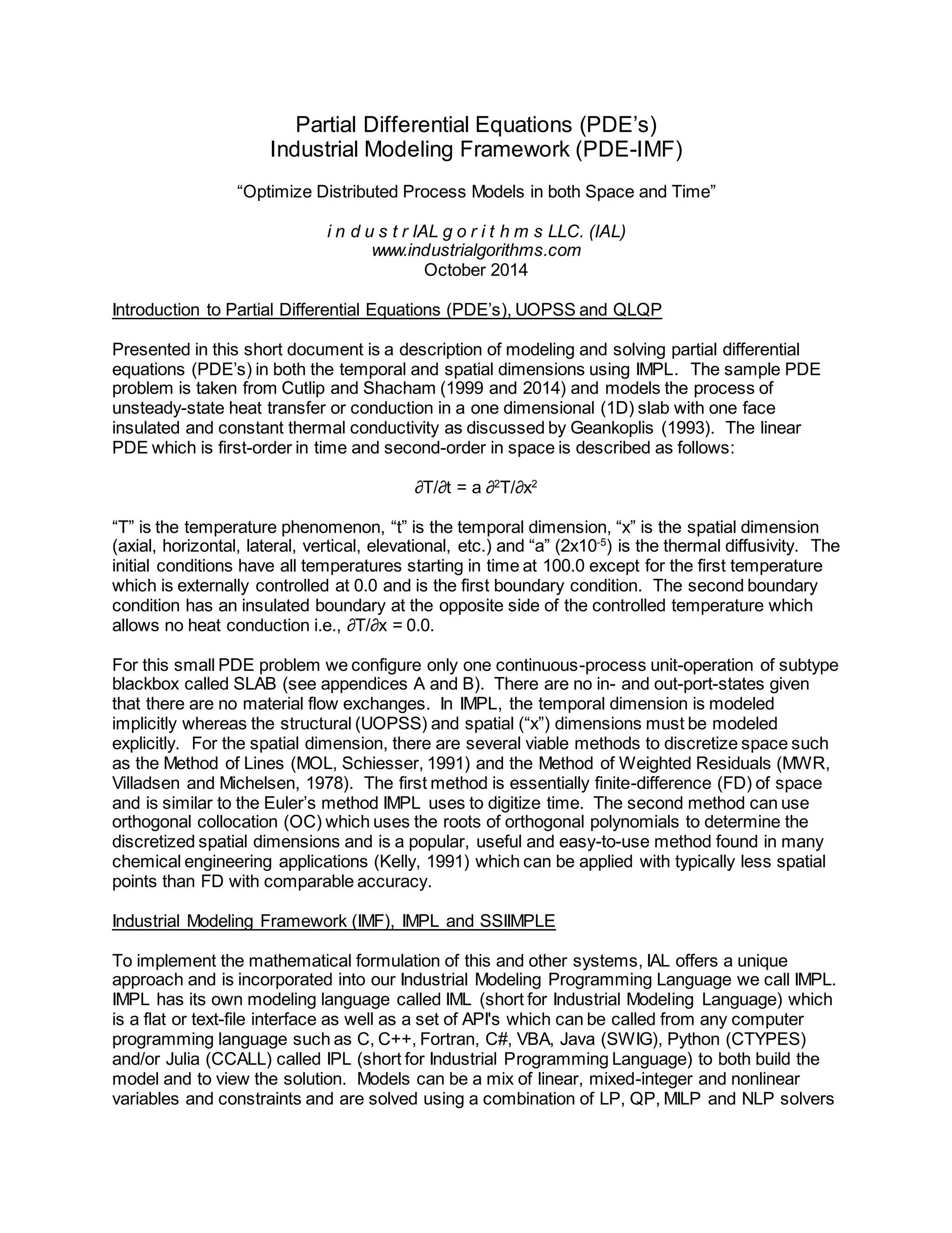
![!!!!!!!!!!!!!!!!!!!!!!!!!!!!!!!!!!!!!!!!!!!!!!!!!!!!!!!!!!!!!!!!!!!!!!!!!!!!!!!!
&sCalc,@sValue
PERIOD,1.0
START,-PERIOD
BEGIN,0.0
END,6000.0
dx,0.1
&sCalc,@sValue
!!!!!!!!!!!!!!!!!!!!!!!!!!!!!!!!!!!!!!!!!!!!!!!!!!!!!!!!!!!!!!!!!!!!!!!!!!!!!!!!
! Chronological Data (Periods)
!!!!!!!!!!!!!!!!!!!!!!!!!!!!!!!!!!!!!!!!!!!!!!!!!!!!!!!!!!!!!!!!!!!!!!!!!!!!!!!!
@rPastTHD,@rFutureTHD,@rTPD
START,END,PERIOD
@rPastTHD,@rFutureTHD,@rTPD
!!!!!!!!!!!!!!!!!!!!!!!!!!!!!!!!!!!!!!!!!!!!!!!!!!!!!!!!!!!!!!!!!!!!!!!!!!!!!!!!
! Construction Data (Pointers)
!!!!!!!!!!!!!!!!!!!!!!!!!!!!!!!!!!!!!!!!!!!!!!!!!!!!!!!!!!!!!!!!!!!!!!!!!!!!!!!!
&sUnit,&sOperation,@sType,@sSubtype,@sUse
SLAB,,processc,blackbox,,
&sUnit,&sOperation,@sType,@sSubtype,@sUse
!!!!!!!!!!!!!!!!!!!!!!!!!!!!!!!!!!!!!!!!!!!!!!!!!!!!!!!!!!!!!!!!!!!!!!!!!!!!!!!!
! Condition Data (Properties)
!!!!!!!!!!!!!!!!!!!!!!!!!!!!!!!!!!!!!!!!!!!!!!!!!!!!!!!!!!!!!!!!!!!!!!!!!!!!!!!!
&sCondition
T1
T2
T3
T4
T5
T6
T7
T8
T9
T10
T11
eqT2
eqT3
eqT4
eqT5
eqT6
eqT7
eqT8
eqT9
eqT10
&sCondition
&sCoefficient,@sType,@sPath_Name,@sLibrary_Name,@sFunction_Name,@iNumber_Conditions,@rPerturb_Size,@sCondition_Names
a,static
&sCoefficient,@sType,@sPath_Name,@sLibrary_Name,@sFunction_Name,@iNumber_Conditions,@rPerturb_Size,@sCondition_Names
&sUnit,&sOperation,&sCondition,@rCondition_Lower,@rCondition_Upper,@rCondition_Target
SLAB,,T1,0.0,0.0,
SLAB,,T2,0.0,200.0,
SLAB,,T3,0.0,200.0,
SLAB,,T4,0.0,200.0,
SLAB,,T5,0.0,200.0,
SLAB,,T6,0.0,200.0,
SLAB,,T7,0.0,200.0,
SLAB,,T8,0.0,200.0,
SLAB,,T9,0.0,200.0,
SLAB,,T10,0.0,200.0,
SLAB,,T11,0.0,200.0,
SLAB,,eqT2,0.0,0.0,
SLAB,,eqT3,0.0,0.0,
SLAB,,eqT4,0.0,0.0,
SLAB,,eqT5,0.0,0.0,
SLAB,,eqT6,0.0,0.0,
SLAB,,eqT7,0.0,0.0,
SLAB,,eqT8,0.0,0.0,
SLAB,,eqT9,0.0,0.0,
SLAB,,eqT10,0.0,0.0,
&sUnit,&sOperation,&sCondition,@rCondition_Lower,@rCondition_Upper,@rCondition_Target
&sUnit,&sOperation,&sCoefficient,@rCoefficient_Lower,@rCoefficient_Upper,@rCoefficient_Target
SLAB,,a,2.0E-5,2.0E-5,
&sUnit,&sOperation,&sCoefficient,@rCoefficient_Lower,@rCoefficient_Upper,@rCoefficient_Target
ConditionsUOCondition-&sUnit,&sOperation,&sCondition,@sType,@rValue,@sValue
SLAB,,eqT2,?,3,T2 - T2[-1] - a / dx^2.0 * (T3-2.0*T2+T1) * PERIOD
SLAB,,eqT3,?,3,T3 - T3[-1] - a / dx^2.0 * (T4-2.0*T3+T2) * PERIOD
SLAB,,eqT4,?,3,T4 - T4[-1] - a / dx^2.0 * (T5-2.0*T4+T3) * PERIOD
SLAB,,eqT5,?,3,T5 - T5[-1] - a / dx^2.0 * (T6-2.0*T5+T4) * PERIOD
SLAB,,eqT6,?,3,T6 - T6[-1] - a / dx^2.0 * (T7-2.0*T6+T5) * PERIOD
SLAB,,eqT7,?,3,T7 - T7[-1] - a / dx^2.0 * (T8-2.0*T7+T6) * PERIOD
SLAB,,eqT8,?,3,T8 - T8[-1] - a / dx^2.0 * (T9-2.0*T8+T7) * PERIOD](https://image.slidesharecdn.com/pde-imf-141015202943-conversion-gate01/75/Partial-Differential-Equations-PDE-s-Industrial-Modeling-Framework-PDE-IMF-5-2048.jpg)
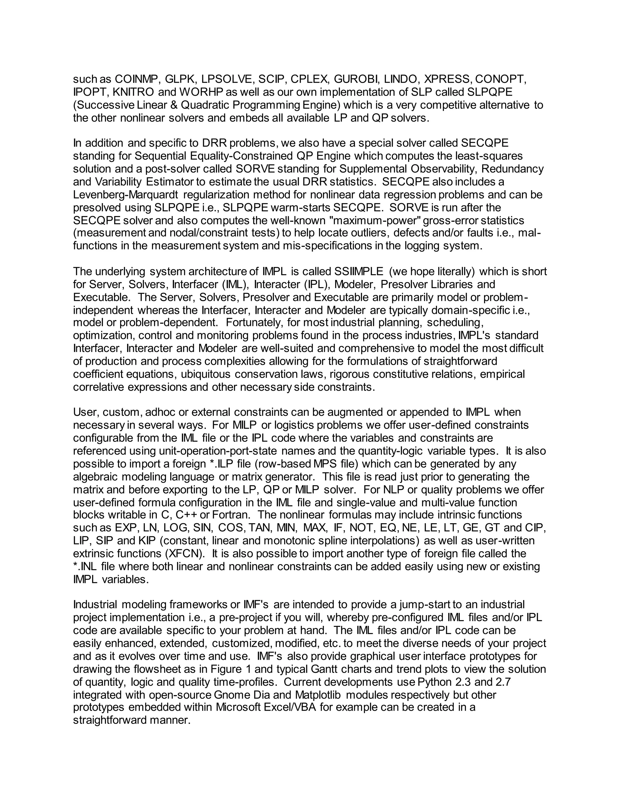
![SLAB,,eqT9,?,3,T9 - T9[-1] - a / dx^2.0 * (T10-2.0*T9+T8) * PERIOD
SLAB,,eqT10,?,3,T10 - T10[-1] - a / dx^2.0 * (T11-2.0*T10+T9) * PERIOD
SLAB,,T11,?,3,(4.0 * T10 - T9) / 3.0
ConditionsUOCondition-&sUnit,&sOperation,&sCondition,@sType,@rValue,@sValue
!!!!!!!!!!!!!!!!!!!!!!!!!!!!!!!!!!!!!!!!!!!!!!!!!!!!!!!!!!!!!!!!!!!!!!!!!!!!!!!!
! Cost Data (Pricing)
!!!!!!!!!!!!!!!!!!!!!!!!!!!!!!!!!!!!!!!!!!!!!!!!!!!!!!!!!!!!!!!!!!!!!!!!!!!!!!!!
&sUnit,&sOperation,&sCondition,@rConditionPro_Weight,@rConditionPer1_Weight,@rConditionPer2_Weight,@rConditionPen_Weight
&sUnit,&sOperation,&sCondition,@rConditionPro_Weight,@rConditionPer1_Weight,@rConditionPer2_Weight,@rConditionPen_Weight
!!!!!!!!!!!!!!!!!!!!!!!!!!!!!!!!!!!!!!!!!!!!!!!!!!!!!!!!!!!!!!!!!!!!!!!!!!!!!!!!
! Content Data (Past, Present Provisos)
!!!!!!!!!!!!!!!!!!!!!!!!!!!!!!!!!!!!!!!!!!!!!!!!!!!!!!!!!!!!!!!!!!!!!!!!!!!!!!!!
&sUnit,&sOperation,&sCondition,@rCondition_Value,@rStart_Time
SLAB,,T2,100.0,0.0
SLAB,,T3,100.0,0.0
SLAB,,T4,100.0,0.0
SLAB,,T5,100.0,0.0
SLAB,,T6,100.0,0.0
SLAB,,T7,100.0,0.0
SLAB,,T8,100.0,0.0
SLAB,,T9,100.0,0.0
SLAB,,T10,100.0,0.0
&sUnit,&sOperation,&sCondition,@rCondition_Value,@rStart_Time
!!!!!!!!!!!!!!!!!!!!!!!!!!!!!!!!!!!!!!!!!!!!!!!!!!!!!!!!!!!!!!!!!!!!!!!!!!!!!!!!
! Command Data (Future Provisos)
!!!!!!!!!!!!!!!!!!!!!!!!!!!!!!!!!!!!!!!!!!!!!!!!!!!!!!!!!!!!!!!!!!!!!!!!!!!!!!!!
&sUnit,&sOperation,@rSetup_Lower,@rSetup_Upper,@rBegin_Time,@rEnd_Time
SLAB,,1,1,BEGIN,END
&sUnit,&sOperation,@rSetup_Lower,@rSetup_Upper,@rBegin_Time,@rEnd_Time
Appendix B – PDE-IMF-OC.IML File
i M P l (c)
Copyright and Property of i n d u s t r I A L g o r i t h m s LLC.
!!!!!!!!!!!!!!!!!!!!!!!!!!!!!!!!!!!!!!!!!!!!!!!!!!!!!!!!!!!!!!!!!!!!!!!!!!!!!!!!
! Calculation Data (Parameters)
!!!!!!!!!!!!!!!!!!!!!!!!!!!!!!!!!!!!!!!!!!!!!!!!!!!!!!!!!!!!!!!!!!!!!!!!!!!!!!!!
&sCalc,@sValue
PERIOD,1.0
START,-PERIOD
BEGIN,0.0
END,6000.0
&sCalc,@sValue
XFCN-@sPath_Name,@sLibrary_Name,@sFunction_Name
C:IndustrialAlgorithmsProceduresx64Release,xfunc_ocl.dll,xfunc_ocl
XFCN-@sPath_Name,@sLibrary_Name,@sFunction_Name
&sCalc,@sValue
ALPHA,0.0
BETA,0.0
A11,XFCN(1;1;3;1;1;1;ALPHA;BETA)
A12,XFCN(1;2;3;1;1;1;ALPHA;BETA)
A13,XFCN(1;3;3;1;1;1;ALPHA;BETA)
A14,XFCN(1;4;3;1;1;1;ALPHA;BETA)
A15,XFCN(1;5;3;1;1;1;ALPHA;BETA)
A21,XFCN(2;1;3;1;1;1;ALPHA;BETA)
A22,XFCN(2;2;3;1;1;1;ALPHA;BETA)
A23,XFCN(2;3;3;1;1;1;ALPHA;BETA)
A24,XFCN(2;4;3;1;1;1;ALPHA;BETA)
A25,XFCN(2;5;3;1;1;1;ALPHA;BETA)
A31,XFCN(3;1;3;1;1;1;ALPHA;BETA)
A32,XFCN(3;2;3;1;1;1;ALPHA;BETA)
A33,XFCN(3;3;3;1;1;1;ALPHA;BETA)
A34,XFCN(3;4;3;1;1;1;ALPHA;BETA)
A35,XFCN(3;5;3;1;1;1;ALPHA;BETA)
A41,XFCN(4;1;3;1;1;1;ALPHA;BETA)
A42,XFCN(4;2;3;1;1;1;ALPHA;BETA)
A43,XFCN(4;3;3;1;1;1;ALPHA;BETA)
A44,XFCN(4;4;3;1;1;1;ALPHA;BETA)
A45,XFCN(4;5;3;1;1;1;ALPHA;BETA)
A51,XFCN(5;1;3;1;1;1;ALPHA;BETA)
A52,XFCN(5;2;3;1;1;1;ALPHA;BETA)
A53,XFCN(5;3;3;1;1;1;ALPHA;BETA)
A54,XFCN(5;4;3;1;1;1;ALPHA;BETA)
A55,XFCN(5;5;3;1;1;1;ALPHA;BETA)
B11,XFCN(1;1;3;1;1;2;ALPHA;BETA)
B12,XFCN(1;2;3;1;1;2;ALPHA;BETA)
B13,XFCN(1;3;3;1;1;2;ALPHA;BETA)
B14,XFCN(1;4;3;1;1;2;ALPHA;BETA)
B15,XFCN(1;5;3;1;1;2;ALPHA;BETA)
B21,XFCN(2;1;3;1;1;2;ALPHA;BETA)](https://image.slidesharecdn.com/pde-imf-141015202943-conversion-gate01/75/Partial-Differential-Equations-PDE-s-Industrial-Modeling-Framework-PDE-IMF-6-2048.jpg)
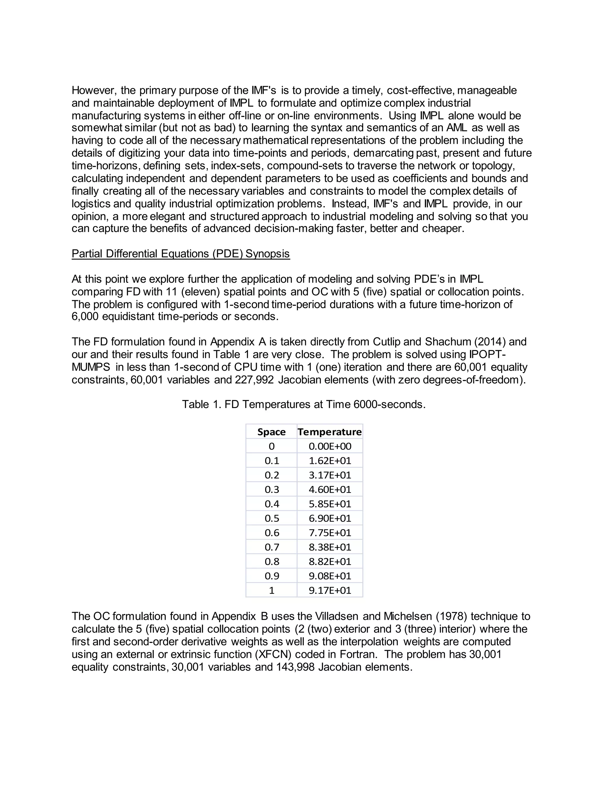
![B22,XFCN(2;2;3;1;1;2;ALPHA;BETA)
B23,XFCN(2;3;3;1;1;2;ALPHA;BETA)
B24,XFCN(2;4;3;1;1;2;ALPHA;BETA)
B25,XFCN(2;5;3;1;1;2;ALPHA;BETA)
B31,XFCN(3;1;3;1;1;2;ALPHA;BETA)
B32,XFCN(3;2;3;1;1;2;ALPHA;BETA)
B33,XFCN(3;3;3;1;1;2;ALPHA;BETA)
B34,XFCN(3;4;3;1;1;2;ALPHA;BETA)
B35,XFCN(3;5;3;1;1;2;ALPHA;BETA)
B41,XFCN(4;1;3;1;1;2;ALPHA;BETA)
B42,XFCN(4;2;3;1;1;2;ALPHA;BETA)
B43,XFCN(4;3;3;1;1;2;ALPHA;BETA)
B44,XFCN(4;4;3;1;1;2;ALPHA;BETA)
B45,XFCN(4;5;3;1;1;2;ALPHA;BETA)
B51,XFCN(5;1;3;1;1;2;ALPHA;BETA)
B52,XFCN(5;2;3;1;1;2;ALPHA;BETA)
B53,XFCN(5;3;3;1;1;2;ALPHA;BETA)
B54,XFCN(5;4;3;1;1;2;ALPHA;BETA)
B55,XFCN(5;5;3;1;1;2;ALPHA;BETA)
C1,XFCN(0.2;1;3;1;1;ALPHA;BETA)
C2,XFCN(0.2;2;3;1;1;ALPHA;BETA)
C3,XFCN(0.2;3;3;1;1;ALPHA;BETA)
C4,XFCN(0.2;4;3;1;1;ALPHA;BETA)
C5,XFCN(0.2;5;3;1;1;ALPHA;BETA)
&sCalc,@sValue
!!!!!!!!!!!!!!!!!!!!!!!!!!!!!!!!!!!!!!!!!!!!!!!!!!!!!!!!!!!!!!!!!!!!!!!!!!!!!!!!
! Chronological Data (Periods)
!!!!!!!!!!!!!!!!!!!!!!!!!!!!!!!!!!!!!!!!!!!!!!!!!!!!!!!!!!!!!!!!!!!!!!!!!!!!!!!!
@rPastTHD,@rFutureTHD,@rTPD
START,END,PERIOD
@rPastTHD,@rFutureTHD,@rTPD
!!!!!!!!!!!!!!!!!!!!!!!!!!!!!!!!!!!!!!!!!!!!!!!!!!!!!!!!!!!!!!!!!!!!!!!!!!!!!!!!
! Construction Data (Pointers)
!!!!!!!!!!!!!!!!!!!!!!!!!!!!!!!!!!!!!!!!!!!!!!!!!!!!!!!!!!!!!!!!!!!!!!!!!!!!!!!!
&sUnit,&sOperation,@sType,@sSubtype,@sUse
SLAB,,processc,blackbox,,
&sUnit,&sOperation,@sType,@sSubtype,@sUse
!!!!!!!!!!!!!!!!!!!!!!!!!!!!!!!!!!!!!!!!!!!!!!!!!!!!!!!!!!!!!!!!!!!!!!!!!!!!!!!!
! Condition Data (Properties)
!!!!!!!!!!!!!!!!!!!!!!!!!!!!!!!!!!!!!!!!!!!!!!!!!!!!!!!!!!!!!!!!!!!!!!!!!!!!!!!!
&sCondition
T1
T2
T3
T4
T5
TX
eqT2
eqT3
eqT4
eqT5
eqTX
&sCondition
&sCoefficient,@sType,@sPath_Name,@sLibrary_Name,@sFunction_Name,@iNumber_Conditions,@rPerturb_Size,@sCondition_Names
a,static
&sCoefficient,@sType,@sPath_Name,@sLibrary_Name,@sFunction_Name,@iNumber_Conditions,@rPerturb_Size,@sCondition_Names
&sUnit,&sOperation,&sCondition,@rCondition_Lower,@rCondition_Upper,@rCondition_Target
SLAB,,T1,0.0,0.0,
SLAB,,T2,0.0,200.0,
SLAB,,T3,0.0,200.0,
SLAB,,T4,0.0,200.0,
SLAB,,T5,0.0,200.0,
SLAB,,TX,0.0,200.0,
SLAB,,eqT2,0.0,0.0,
SLAB,,eqT3,0.0,0.0,
SLAB,,eqT4,0.0,0.0,
SLAB,,eqT5,0.0,0.0,
&sUnit,&sOperation,&sCondition,@rCondition_Lower,@rCondition_Upper,@rCondition_Target
&sUnit,&sOperation,&sCoefficient,@rCoefficient_Lower,@rCoefficient_Upper,@rCoefficient_Target
SLAB,,a,2.0E-5,2.0E-5,
&sUnit,&sOperation,&sCoefficient,@rCoefficient_Lower,@rCoefficient_Upper,@rCoefficient_Target
ConditionsUOCondition-&sUnit,&sOperation,&sCondition,@sType,@rValue,@sValue
SLAB,,eqT2,?,3,T2 - T2[-1] - a * (B21*T1+B22*T2+B23*T3+B24*T4+B25*T5) * PERIOD
SLAB,,eqT3,?,3,T3 - T3[-1] - a * (B31*T1+B32*T2+B33*T3+B34*T4+B35*T5) * PERIOD
SLAB,,eqT4,?,3,T4 - T4[-1] - a * (B41*T1+B42*T2+B43*T3+B44*T4+B45*T5) * PERIOD
SLAB,,eqT5,?,3,(A51*T1+A52*T2+A53*T3+A54*T4+A55*T5)
SLAB,,TX,?,3,(C1*T1+C2*T2+C3*T3+C4*T4+C5*T5)
ConditionsUOCondition-&sUnit,&sOperation,&sCondition,@sType,@rValue,@sValue
!!!!!!!!!!!!!!!!!!!!!!!!!!!!!!!!!!!!!!!!!!!!!!!!!!!!!!!!!!!!!!!!!!!!!!!!!!!!!!!!
! Cost Data (Pricing)
!!!!!!!!!!!!!!!!!!!!!!!!!!!!!!!!!!!!!!!!!!!!!!!!!!!!!!!!!!!!!!!!!!!!!!!!!!!!!!!!](https://image.slidesharecdn.com/pde-imf-141015202943-conversion-gate01/75/Partial-Differential-Equations-PDE-s-Industrial-Modeling-Framework-PDE-IMF-7-2048.jpg)
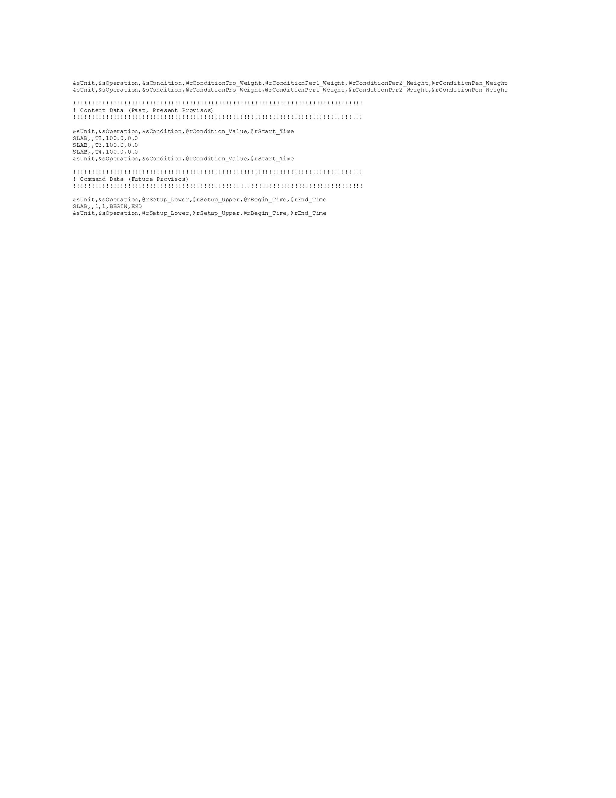

This document discusses modeling and solving partial differential equations (PDEs) using the Industrial Modeling Framework (IMF). It presents a sample 1D heat transfer PDE problem and models it using finite difference (FD) and orthogonal collocation (OC) methods. The results show good agreement between the two methods. IMPL can model both dynamic and spatially distributed problems by discretizing across time and space to obtain algebraic equations that can then be optimized.


![[DSC Europe 25] Marko Krstic - Understanding the AI Threat Landscape - Risks,...](https://cdn.slidesharecdn.com/ss_thumbnails/tiyim1ins5jvbrvzpzla-2-251209104645-c69d3553-thumbnail.jpg?width=640&height=640&fit=bounds)

![[DSC Europe 25] Katherine Forrest - AI NOW: Understanding the Velocity of Cha...](https://cdn.slidesharecdn.com/ss_thumbnails/wvvbruqfrci0sfq9xwgb-4-251212104007-e5ad1987-thumbnail.jpg?width=640&height=640&fit=bounds)
![[DSC Europe 25] Bassam Maharmeh - Artificial Intelligence: Opportunities and ...](https://cdn.slidesharecdn.com/ss_thumbnails/thhfmr2fqpawzj7hsjpg-5-251211083048-2c23204f-thumbnail.jpg?width=640&height=640&fit=bounds)

![[DSC Europe 25] Nikolay Burlutskiy - Best Practices for Building Enterprise M...](https://cdn.slidesharecdn.com/ss_thumbnails/uirvaiuvq8y1w8hzd9tx-7-251212103249-2619edb4-thumbnail.jpg?width=640&height=640&fit=bounds)

![[DSC Europe 25] Sara Polak - The Archaeology of Innovation: AI as the Next Cr...](https://cdn.slidesharecdn.com/ss_thumbnails/7ecbscdnt8mlcuqbd2ln-2-sara-polak-ai-creative-industries-251208152533-aa1fcf54-thumbnail.jpg?width=640&height=640&fit=bounds)
![[DSC Europe 25] Milan Sekuloski - Data, Defence, and Development: Cybersecuri...](https://cdn.slidesharecdn.com/ss_thumbnails/dfrkwwx4qly6atqpbl4z-4-251209104645-c3d4b0ca-thumbnail.jpg?width=640&height=640&fit=bounds)
![[DSC Europe 25] Kaja Kandare - LLM as a judge.pptx](https://cdn.slidesharecdn.com/ss_thumbnails/arxyccaxsdsd1ba99wjw-7-251212104007-2b4e3f64-thumbnail.jpg?width=640&height=640&fit=bounds)
![[DSC Europe 25] Milan Zdravkovic - The road less traveled in District Heating...](https://cdn.slidesharecdn.com/ss_thumbnails/nfaboniqwsz4ucyctnmy-2-milan-zdravkovic-dsc2025-the-road-less-traveled-in-district-heating-operation-251208151905-f56388a5-thumbnail.jpg?width=640&height=640&fit=bounds)
![[DSC Europe 25] Jovan Bogicevic - Legacy to AI-Driven Defense: Transforming D...](https://cdn.slidesharecdn.com/ss_thumbnails/rsarluadt563hntyfc8q-3-251211083849-3e7bc4c0-thumbnail.jpg?width=640&height=640&fit=bounds)

![[DSC Europe 25] Branko Dzakula - From Defense to Attack: How AI Redefines Cyb...](https://cdn.slidesharecdn.com/ss_thumbnails/80bdzdxpr3ky2g0qvyk9-8-251211083048-ce5fc1ee-thumbnail.jpg?width=640&height=640&fit=bounds)


![[DSC Europe 25] Dunja Adzic Jovanovic - AI and Cybersecurity: Defending Data ...](https://cdn.slidesharecdn.com/ss_thumbnails/o1zylpbhrtwnixxq2xj8-7-251211083048-185086f6-thumbnail.jpg?width=640&height=640&fit=bounds)
![[DSC Europe 25] Branko Urosevic -Rethinking Financial Talent: Integrating Cod...](https://cdn.slidesharecdn.com/ss_thumbnails/8jjrus8ttko6qj64f58f-3-251212103250-642c6374-thumbnail.jpg?width=640&height=640&fit=bounds)