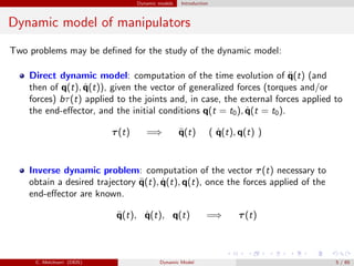
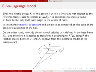
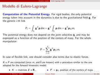
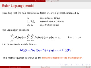
Dynamic models of robot manipulators can be developed using either an Euler-Lagrange approach or a Newton-Euler approach. The Euler-Lagrange approach defines the kinetic and potential energies of each link to obtain the dynamic model analytically. It provides simpler intuition but is less computationally efficient. The Newton-Euler approach uses a recursive technique that exploits the serial structure of manipulators to efficiently compute dynamics in a non-closed form. Both approaches result in the same dynamic model relating joint forces/torques to accelerations.
![Dynamic models Euler-Lagrange model
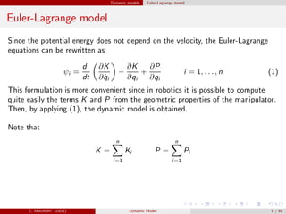
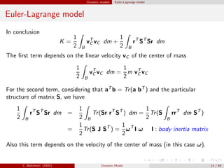
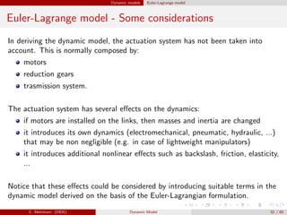
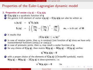
Euler-Lagrange model - Some considerations
The elements of matrix C(q, ˙q) are computed as follows. From
n
i=1
n
j=1
hkji ˙qi ˙qj =
n
i=1
n
j=1
∂Mkj
∂qi
−
1
2
∂Mij
∂qk
˙qi ˙qj
by exchanging the sum (i, j) and exploiting the symmetry one obtains
n
i=1
n
j=1
∂Mkj
∂qi
=
1
2
n
i=1
n
j=1
∂Mkj
∂qi
+
∂Mki
∂qj
and then
n
i=1
n
j=1
∂Mkj
∂qi
−
1
2
∂Mij
∂qk
=
n
i=1
n
j=1
1
2
∂Mkj
∂qi
+
∂Mki
∂qj
−
∂Mij
∂qk
=
n
i=1
n
j=1
cijk
where cijk = 1
2
∂Mkj
∂qi
+ ∂Mki
∂qj
−
∂Mij
∂qk
are the so-called Christoffel Symbols.
Since matrix M(q) is symmetric, for a given k then cijk = cjik .
The elements of matrix C(q, ˙q)are then computed as
[C(q, ˙q)]k,j =
n
i=1
cijk ˙qi (5)
C. Melchiorri (DEIS) Dynamic Model 27 / 65](https://image.slidesharecdn.com/fir05dynamics-150703030454-lva1-app6891/85/Fir-05-dynamics-27-320.jpg)
![Dynamic models Euler-Lagrange model
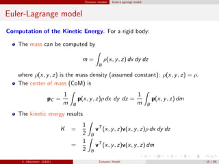
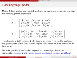
Euler-Lagrange model - Some considerations
This is not the only possible expression for matrix C(q, ˙q). In general, any matrix
such that
n
j=1
cij ˙qj =
n
j=1
n
k=1
hijk ˙qk ˙qj
can be considered. The choice (4) is preferred since in this case the following
property is verified.
Property. Matrix N(q, ˙q), defined as
N(q, ˙q) = ˙M(q, ˙q) − 2C(q, ˙q) (6)
in which the elements of C(q, ˙q) are defined as
cijk =
1
2
∂Mkj
∂qi
+
∂Mki
∂qj
−
∂Mij
∂qk
[C(q, ˙q)]k,j =
n
i=1
cijk ˙qi
results skew-symmetric, i.e. nkj = −njk , nkk = 0.
C. Melchiorri (DEIS) Dynamic Model 28 / 65](https://image.slidesharecdn.com/fir05dynamics-150703030454-lva1-app6891/85/Fir-05-dynamics-28-320.jpg)
![Dynamic models Euler-Lagrange model
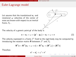
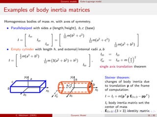
Euler-Lagrange model - Some considerations
In fact, by considering the generic element nkj , one obtains
nkj =
d Mkj
dt
− 2[C]kj
=
n
i=1
∂Mkj
∂qi
− (
∂Mkj
∂qi
+
∂Mki
∂qj
−
∂Mij
∂qk
) ˙qi
=
n
i=1
∂Mij
∂qk
−
∂Mki
∂qj
˙qi
from which it follows (if indices k and j are exchanged, because of the symmetry
of M(q)) that nkj = −njk .
Since matrix N is skew-symmetrix, then
xT
N(q, ˙q) x = 0, ∀x
C. Melchiorri (DEIS) Dynamic Model 29 / 65](https://image.slidesharecdn.com/fir05dynamics-150703030454-lva1-app6891/85/Fir-05-dynamics-29-320.jpg)
![Dynamic models Euler-Lagrange model
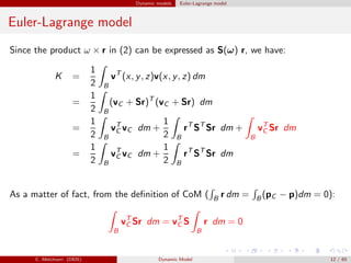
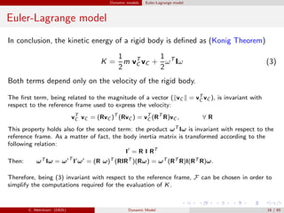
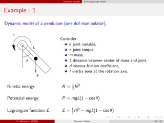
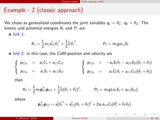
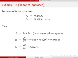
Example - 2 (classic approach)
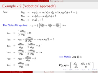
Therefore, L = K1 + K2 − P1 − P2 and
τ1 = [m1a2
C1 + ˜I1 + m2(a2
1 + a2
C2 + 2a1aC2C2) + ˜I2]¨θ1 +
+[m2(a2
C2 + a1aC2C2) + ˜I2]¨θ2 − m2a1aC2S2(2 ˙θ1
˙θ2 + ˙θ2
2) +
+m1gaC1C1 + m2g(a1C1 + aC2C12)
τ2 = [m2(a2
C2 + a1aC2C2) + ˜I2] ¨θ1 + (m2a2
C2 + ˜I2)¨θ2 +
m2a1aC2S2
˙θ2
1 + m2gaC2C12
C. Melchiorri (DEIS) Dynamic Model 37 / 65](https://image.slidesharecdn.com/fir05dynamics-150703030454-lva1-app6891/85/Fir-05-dynamics-37-320.jpg)
![Dynamic models Euler-Lagrange model
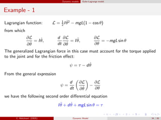
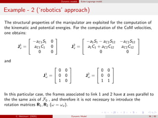
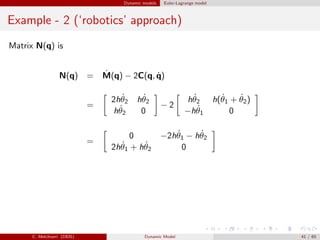
Example - 2 (‘robotics’ approach)
Summarizing, we have
M11
¨θ1 + M12
¨θ2 + c121
˙θ1
˙θ2 + c211
˙θ2
˙θ1 + c221
˙θ2
2 + g1 = τ1
M21
¨θ1 + M22
¨θ2 + c112
˙θ2
1 + g2 = τ2
or
[m1a2
C1 + m2(a2
1 + a2
C2 + 2a1aC2C2) + ˜I1 + ˜I2]¨θ1 + [m2(a2
C2 + a1a2
C2C2) + ˜I2]¨θ2
−m2a1aC2S2
˙θ2
2 − 2m2a1aC2S2
˙θ1
˙θ2
+(m1aC1 + m2a1)gC1 + m2gaC2C12 = τ1
[m2(a2
C2 + a1aC2C2) + ˜I2]¨θ1 + [m2a2
C2 + ˜I2]¨θ2
+m2a1aC2S2
˙θ2
1
+m2gaC2C12 = τ2
=⇒ Same result!
C. Melchiorri (DEIS) Dynamic Model 43 / 65](https://image.slidesharecdn.com/fir05dynamics-150703030454-lva1-app6891/85/Fir-05-dynamics-43-320.jpg)
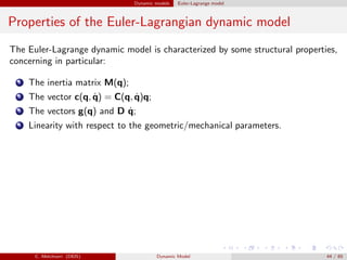
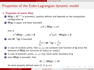
![Dynamic models Euler-Lagrange model
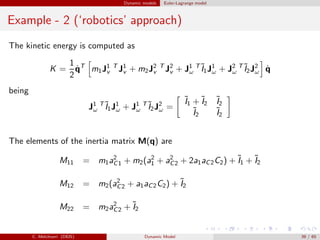
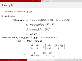
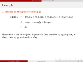
Example
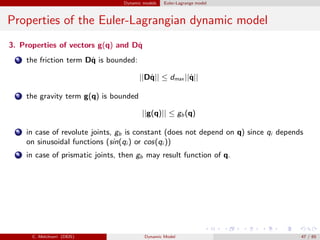
Properties of the dynamic model of a
2 dof manipulator.
Neglecting friction effects we have:
M(q) =
m1a2
C1 + m2(a2
1 + a2
C2 + 2a1aC2C2) + ˜I1 + ˜I2 m2(a2
C2 + a1aC2C2) + ˜I2
m2(a2
C2 + a1aC2C2) + ˜I2 m2a2
C2 + ˜I2
C(q, ˙q)˙q = −m2a1aC2S2
2 ˙θ1
˙θ2 + ˙θ2
2
− ˙θ2
1
, g(q)=
(m1aC1 + m2a1)gC1 + m2gaC2C12
m2gaC2C12
Consider (for the sake of simplicity) the 1-norm || · ||1, and θ1, θ2 ∈ [−π/2, π/2].
C. Melchiorri (DEIS) Dynamic Model 49 / 65](https://image.slidesharecdn.com/fir05dynamics-150703030454-lva1-app6891/85/Fir-05-dynamics-49-320.jpg)
![Dynamic models Euler-Lagrange model
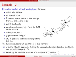
Example
Plots of the eigenvalues of M(q) for the 2 dof planar manipulator
0
50
100
150
200
250
300
350
0
100
200
300
400
0
20
40
60
80
100
120
140
160
180
l
m
in = 6.2399
l
m
ax = 161.2601
q1 [deg]
Andamento autovalori minimo e massimo di M(q)
q2 [deg]
λmin = 6.2399
λmax = 161.2601
In this case, the eigenvalues depend only on q2! These results have been obtained
with:
m1 = m2 = 50kg; I1 = I2 = 10; a1 = a2 = 1; ac1 = ac2 = 0.5
One obtains
M1 = 117, 5, M2 = 192.5 e M 1 = 192.5, M 2 = 161.26, M ∞ = 192.5
C. Melchiorri (DEIS) Dynamic Model 53 / 65](https://image.slidesharecdn.com/fir05dynamics-150703030454-lva1-app6891/85/Fir-05-dynamics-53-320.jpg)
![Dynamic models Euler-Lagrange model
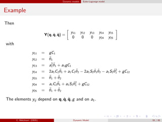
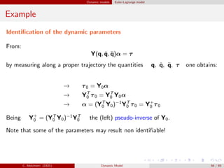
Example
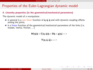
3. Linearity of the dynamic model Y(q, ˙q, ¨q)α = τ
[m1a2
C1 + m2(a2
1 + a2
C2 + 2a1aC2C2) + ˜I1 + ˜I2]¨θ1 + [m2(a2
C2 + a1a2
C2C2) + ˜I2]¨θ2
−m2a1aC2S2
˙θ2
2 − 2m2a1aC2S2
˙θ1
˙θ2
+(m1aC1 + m2a1)gC1 + m2gaC2C12 = τ1
[m2(a2
C2 + a1aC2C2) + ˜I2]¨θ1 + [m2a2
C2 + ˜I2]¨θ2
+m2a1aC2S2
˙θ2
1
+m2gaC2C12 = τ2
By inspection, one can define the parameters vector
α = [α1, α2, α3, α4, α5]T
with
α1 = m1aC1, α2 = m1a2
C1 + ˜I1, α3 = m2, α4 = m2aC2, α5 = m2a2
C2 + ˜I2
C. Melchiorri (DEIS) Dynamic Model 54 / 65](https://image.slidesharecdn.com/fir05dynamics-150703030454-lva1-app6891/85/Fir-05-dynamics-54-320.jpg)
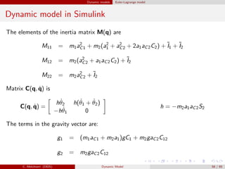
![Dynamic models Euler-Lagrange model
Dynamic model in Simulink
%%%%% Elements of the Inertia Matrix M
M11 = I1z+I2z+Lg1^2*m1+m2*(L1^2+Lg2^2+2*L1*Lg2*c2);
M12 = I2z+m2*(Lg2^2+L1*Lg2*c2);
M22 = I2z+Lg2^2*m2;
M = [M11, M12; M12, M22];
%%%%% Coriolis and centrifugal elements
C11 = -(L1*dq2*s2*(Lg2*m2)); C12 = -(L1*dq12*s2*(Lg2*m2));
C21 = m2*L1*Lg2*s2*dq1; C22 = 0;
C = [C11 C12; C21 C22];
%%%%% Gravity :
g1 = m1*Lg1*c1+m2*(Lg2*c12 + L1*c1); g2 = m2*Lg2*c12;
G = g*[g1; g2];
%%%%% Computation of acceleration
ddq = inv(M) * (tau + tauint - C*dq - D*dq - G);
C. Melchiorri (DEIS) Dynamic Model 60 / 65](https://image.slidesharecdn.com/fir05dynamics-150703030454-lva1-app6891/85/Fir-05-dynamics-60-320.jpg)
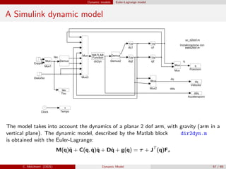
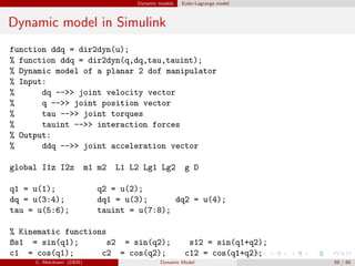
![Dynamic models Euler-Lagrange model
Dynamic model in Simulink
% Simulation of the dynamic model of a planar 2 dof manipulator
% Simulink scheme: sc_d2dof.m
% Definition and initialization of global variables
% Run the simulation RK45
%
%%%%%%%%%%%%%%%%%%%%%%%%%%%%%%
%%%% Robots’ Coefficients %%%%
%%%%%%%%%%%%%%%%%%%%%%%%%%%%%%
clear I1z I2z m1 m2 L1 L2 Lg1 Lg2 g D
global I1z I2z m1 m2 L1 L2 Lg1 Lg2 g D
I1z = 10; I2z = 10;
m1 = 50.0; m2 = 50.0;
L1 = 1; L2 = 1;
Lg1=L1/2; Lg2=L2/2;
g = 9.81;
D = 0.0 * eye(2); % friction
% D = diag([30,30]); % friction
% D = diag([80,80]); % friction
C. Melchiorri (DEIS) Dynamic Model 61 / 65](https://image.slidesharecdn.com/fir05dynamics-150703030454-lva1-app6891/85/Fir-05-dynamics-61-320.jpg)
![Dynamic models Euler-Lagrange model
Dynamic model in Simulink
COPPIA = 0; % joint torques
DISTURBO = 0; % joint torques due to interaction with environment
%%%% Iniziatialization and run
TI = 0; TF = 10;
ERR = 1e-3;
TMIN = 0.002; TMAX = 10*TMIN;
OPTIONS = [ERR,TMIN,TMAX,0,0,2];
X0 = [0 0 0 0];
[ti,xi,yi]=rk45(’sc_d2dof’,TF,X0,OPTIONS);
C. Melchiorri (DEIS) Dynamic Model 62 / 65](https://image.slidesharecdn.com/fir05dynamics-150703030454-lva1-app6891/85/Fir-05-dynamics-62-320.jpg)
![Dynamic models Euler-Lagrange model
Dynamic model in Simulink
D = diag[0, 0];
0 1 2 3 4 5 6 7 8 9 10
−4
−3
−2
−1
0
1
Posizioni q1, q2 (dash)
0 1 2 3 4 5 6 7 8 9 10
−10
−5
0
5
10
Velocita‘ dq1, dq2 (dash)
0 1 2 3 4 5 6 7 8 9 10
−40
−20
0
20
40
Accelerazioni ddq1, ddq2 (dash)
0 1 2 3 4 5 6 7 8 9 10
−1
−0.5
0
0.5
1
Coppie tau1, tau2 (dash)
C. Melchiorri (DEIS) Dynamic Model 63 / 65](https://image.slidesharecdn.com/fir05dynamics-150703030454-lva1-app6891/85/Fir-05-dynamics-63-320.jpg)
![Dynamic models Euler-Lagrange model
Dynamic model in Simulink
D = diag[30, 30];
0 1 2 3 4 5 6 7 8 9 10
−3
−2
−1
0
1
Posizioni q1, q2 (dash)
0 1 2 3 4 5 6 7 8 9 10
−4
−2
0
2
4
Velocita‘ dq1, dq2 (dash)
0 1 2 3 4 5 6 7 8 9 10
−15
−10
−5
0
5
10
15
Accelerazioni ddq1, ddq2 (dash)
0 1 2 3 4 5 6 7 8 9 10
−1
−0.5
0
0.5
1
Coppie tau1, tau2 (dash)
C. Melchiorri (DEIS) Dynamic Model 64 / 65](https://image.slidesharecdn.com/fir05dynamics-150703030454-lva1-app6891/85/Fir-05-dynamics-64-320.jpg)
![Dynamic models Euler-Lagrange model
Dynamic model in Simulink
D = diag[80, 80];
0 1 2 3 4 5 6 7 8 9 10
−3
−2
−1
0
1
2
Velocita‘ dq1, dq2 (dash)
0 1 2 3 4 5 6 7 8 9 10
−3
−2
−1
0
1
Posizioni q1, q2 (dash)
0 1 2 3 4 5 6 7 8 9 10
−15
−10
−5
0
5
10
15
Accelerazioni ddq1, ddq2 (dash)
0 1 2 3 4 5 6 7 8 9 10
−1
−0.5
0
0.5
1
Coppie tau1, tau2 (dash)
C. Melchiorri (DEIS) Dynamic Model 65 / 65](https://image.slidesharecdn.com/fir05dynamics-150703030454-lva1-app6891/85/Fir-05-dynamics-65-320.jpg)