This thesis derives the dynamic model of an industrial robot manipulator using the Newton-Euler formulation. The manipulator studied is an ABB IRB 140 with 6 degrees of freedom recently acquired by NTNU. The objectives are to research the Newton-Euler method, derive the dynamic model of the IRB 140 in an automated way, simulate the model in open and closed loop, and compare results to a model derived using Euler-Lagrange formulation. The thesis contributes an automated framework for applying Newton-Euler formulation to any serial manipulator. Simulations show the open loop system is unstable but achieves stability with PD control and gravity compensation. Computation time is significantly less for Newton-Euler compared to treating the full system with Euler-

1. Master of Science in Engineering Cybernetics
June 2011
Jan Tommy Gravdahl, ITK
Submission date:
Supervisor:
Norwegian University of Science and Technology
Department of Engineering Cybernetics
Dynamic Modeling and Simulation of
Robot Manipulators
The Newton-Euler Formulation
Herman Høifødt

3. NTNU Fakultet for informasjonsteknologi,
Norges teknisk-naturvitenskapelige matematikk og elektroteknikk
universitet Institutt for teknisk kybernetikk
0BMSc thesis assignment
Name of the candidate: Herman Høifødt
Subject: Engineering Cybernetics
Title: Dynamic Modeling and Simulation of Robot Manipulators: The Newton-
Euler Formulation
1BBackground
ABB has produced an industrial robot manipulator called IRB 140. The Department of Engineering
Cybernetics at NTNU recently acquired one of these manipulators to do research in robotics, as well
as to use it in student lab exercises.
As a continuation of the project work1
, the student will derive a complete dynamic model of the
manipulator by the Newton-Euler formulation.
Assignment:
1. Research dynamic modeling of robot manipulators with particular focus on the Newton-Euler
formulation.
2. Search the manipulator datasheets for information that is applicable to the modeling and
perform parameter estimation when required.
3. Based on the Newton-Euler formulation, choose an appropriate software tool and design an
automated framework for deriving the dynamic model of any serial robot manipulator with
revolute joints.
4. Derive the dynamic model for the IRB 140.
5. Simulate the dynamic model in open loop and investigate the energy properties of the model.
6. Perform simulations of position control with a multivariable PD-controller.
7. Compare characteristics of the dynamic model with the dynamic model of the same
manipulator derived by the Euler-Lagrange formulation2
.
To be handed in by: 27/6-2011
Trondheim, 24.01.2011
_____________________ _____________________
Jan Tommy Gravdahl Uwe Mettin
Professor, supervisor Post.doc, advisor
1
H.Høifødt. Dynamics of robot manipulators by the Newton-Euler forumlation , 5th
year project work, 2010.
2
Work done by PhD stduent S. Pchelkin.

5. Abstract
Dynamic modeling means deriving equations that explicitly describes the rela-
tionship between force and motion in a system. To be able to control a robot
manipulator as required by its operation, it is important to consider the dynamic
model in design of the control algorithm and simulation of motion.
In general there are two approaches available; the Euler-Lagrange formula-
tion and the Newton-Euler formulation. This thesis explains briey the dier-
ences of the formulations, and then research the Newton-Euler method in detail.
A complete derivation of the method is derived, and an automated framework
for applying the method on any serial manipulator with revolute joints is pre-
sented.
By using the framework, the Newton-Euler formulation is applied on a mod-
ern industrial manipulator with six degrees of freedom. The dynamic param-
eters of the system are estimated, and the validity of the resulting dynamic
model is veried by several simulations in open and closed loop.
The simulations show that the system is unstable in open loop, and that it
achieves global asymptotic stability in closed loop with gravity compensation,
by including PD controllers with independent joint control. The latter is a con-
rmation of a mathematical proof based on a Lyapunov stability analysis, which
is presented as well. Equivalent simulations of the dynamic model of the same
manipulator derived by the standard Euler-Lagrange formulation show that the
eciency of recursive procedures is way higher that treating the manipulator
as a whole.
A suggestion for future work is performing thorough dynamic parameter
identication. An improved model can ultimately be implemented in the con-
troller of the manipulator, and optimized for a specic job task.

7. Preface
This thesis presents the work from the nal semester of my Master of Engineer-
ing Cybernetics education at the Norwegian University of Science and Technol-
ogy (NTNU). The topic of the work is dynamic modeling of robot manipulators,
where the dynamic model of an industrial manipulator recently acquired by The
Department of Engineering Cybernetics has been derived by the Newton-Euler
formulation.
I am very grateful for the support from supervisor Jan Tommy Gravdahl,
who recommended me to the subject of robotics and gave me the opportunity to
research this manipulator. Our regularly meetings have encouraged me through
the whole work, and his advices and ideas have been very helpful.
I would also like to thank my advisor Uwe Mettin who has supported me
in several modeling challenges during the project. His expertise in robotics and
control engineering has been much appreciated.
In the end I would like to thank my fellow co-students for a great time this
semester. The numerous hours and days at the oce would not have been the
same without their help and our social environment.
Trondheim, June 2011
Herman Høifødt
iii

9. Contents
Abstract i
Preface iii
List of Figures vi
1 Introduction 1
1.1 History and Motivation . . . . . . . . . . . . . . . . . . . . . . . 1
1.2 The IRB 140 . . . . . . . . . . . . . . . . . . . . . . . . . . . . . 2
1.3 Objective . . . . . . . . . . . . . . . . . . . . . . . . . . . . . . . 2
1.4 Software . . . . . . . . . . . . . . . . . . . . . . . . . . . . . . . . 3
1.5 Outline . . . . . . . . . . . . . . . . . . . . . . . . . . . . . . . . 4
1.6 Contributions . . . . . . . . . . . . . . . . . . . . . . . . . . . . . 5
2 Background Theory and Notation 7
2.1 The Rotation Matrix . . . . . . . . . . . . . . . . . . . . . . . . . 7
2.1.1 Vectors and Rotational Transformations . . . . . . . . . . 8
2.1.2 Properties of the Rotation Matrices . . . . . . . . . . . . 8
2.1.3 Relation to Skew Symmetric Matrices . . . . . . . . . . . 8
2.2 Kinematic Chains . . . . . . . . . . . . . . . . . . . . . . . . . . . 9
2.3 The Inertia Tensor . . . . . . . . . . . . . . . . . . . . . . . . . . 11
2.4 Feedback Controllers . . . . . . . . . . . . . . . . . . . . . . . . . 11
2.5 Positive and Negative Deniteness . . . . . . . . . . . . . . . . . 12
3 Dynamic Modeling of Robot Manipulators in General 13
3.1 Dierent Approaches . . . . . . . . . . . . . . . . . . . . . . . . . 13
3.1.1 Euler-Lagrange versus Newton-Euler . . . . . . . . . . . . 14
3.1.2 Dynamic Parameter Identication . . . . . . . . . . . . . 15
3.2 Derivation of the Newton-Euler Formulation . . . . . . . . . . . . 15
3.2.1 The General Case . . . . . . . . . . . . . . . . . . . . . . 16
3.2.2 Equations of an n-link Manipulator . . . . . . . . . . . . 17
3.2.3 Automated Framework . . . . . . . . . . . . . . . . . . . . 20
v

10. 4 System Description and Dynamic Parameter Estimation 23
4.1 Information from Data Sheets . . . . . . . . . . . . . . . . . . . . 23
4.2 Limitations . . . . . . . . . . . . . . . . . . . . . . . . . . . . . . 24
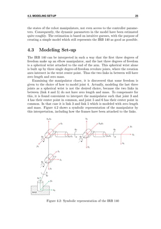
4.3 Modeling Set-up . . . . . . . . . . . . . . . . . . . . . . . . . . . 25
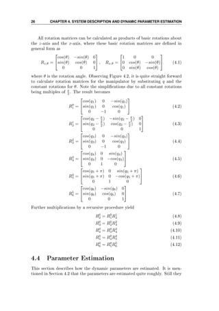
4.4 Parameter Estimation . . . . . . . . . . . . . . . . . . . . . . . . 26
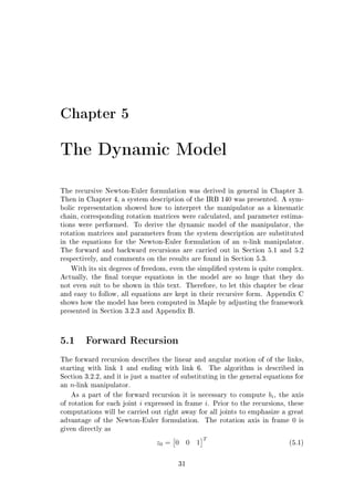
5 The Dynamic Model 31
5.1 Forward Recursion . . . . . . . . . . . . . . . . . . . . . . . . . . 31
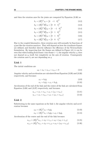
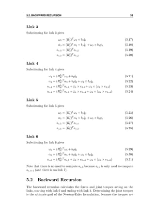
5.2 Backward Recursion . . . . . . . . . . . . . . . . . . . . . . . . . 33
5.3 Comments . . . . . . . . . . . . . . . . . . . . . . . . . . . . . . . 35
6 Simulations and Results 37
6.1 Simulation Structure . . . . . . . . . . . . . . . . . . . . . . . . . 37
6.2 Reduced System Order . . . . . . . . . . . . . . . . . . . . . . . . 38
6.3 Open Loop with Desired Torque . . . . . . . . . . . . . . . . . . 39
6.3.1 Simulations . . . . . . . . . . . . . . . . . . . . . . . . . . 39
6.3.2 Comments . . . . . . . . . . . . . . . . . . . . . . . . . . . 41
6.4 Energy Properties . . . . . . . . . . . . . . . . . . . . . . . . . . 44
6.4.1 Kinetic Energy . . . . . . . . . . . . . . . . . . . . . . . . 44
6.4.2 Potential Energy . . . . . . . . . . . . . . . . . . . . . . . 44
6.4.3 Pendulum Comparison . . . . . . . . . . . . . . . . . . . . 45
6.4.4 Simulations . . . . . . . . . . . . . . . . . . . . . . . . . . 45
6.4.5 Comments . . . . . . . . . . . . . . . . . . . . . . . . . . . 46
6.5 Closed Loop Position Control . . . . . . . . . . . . . . . . . . . . 49
6.5.1 Proof: PD control with gravity compensation . . . . . . . 49
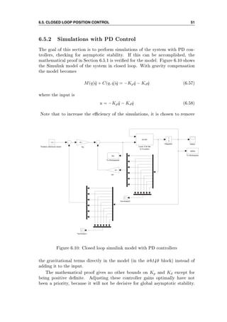
6.5.2 Simulations with PD Control . . . . . . . . . . . . . . . . 51
6.5.3 Comments and Limitations . . . . . . . . . . . . . . . . . 53
7 Comparing the Results to the Euler-Lagrange Model 59
7.1 Remarks on the Direction of State Variables . . . . . . . . . . . . 59
7.2 Computation Times . . . . . . . . . . . . . . . . . . . . . . . . . 62
7.2.1 Open Loop . . . . . . . . . . . . . . . . . . . . . . . . . . 62
7.2.2 Closed loop . . . . . . . . . . . . . . . . . . . . . . . . . . 62
7.2.3 Comments . . . . . . . . . . . . . . . . . . . . . . . . . . . 63
8 Concluding Remarks 65
8.1 Conclusion . . . . . . . . . . . . . . . . . . . . . . . . . . . . . . 65
8.2 Recommendations for Future Work . . . . . . . . . . . . . . . . . 66
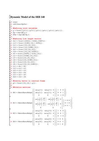
A IRB 140 Data Sheet 67
B Automated Framework 71
C IRB 140 Dynamic Model 77
D Errata in Chapter 7.6 in [20] 105
E Contents of Attached ZIP-File 109
vi

11. List of Figures
1.1 The IRB 140 with its six degrees of freedom [16] . . . . . . . . . 3
2.1 Symbolic representation of robot joints [20] . . . . . . . . . . . . 9
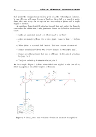
2.2 Links, joints and coordinate frames on an elbow manipulator . . 10
3.1 Forces and torques acting on a random link . . . . . . . . . . . . 18
4.1 View of the manipulator from the back and side [16] . . . . . . . 24
4.2 Symbolic representation of the IRB 140 . . . . . . . . . . . . . . 25
4.3 The centers of mass from the back and side [16] . . . . . . . . . . 27
4.4 Example of link 2 modeled as a cylinder . . . . . . . . . . . . . . 28
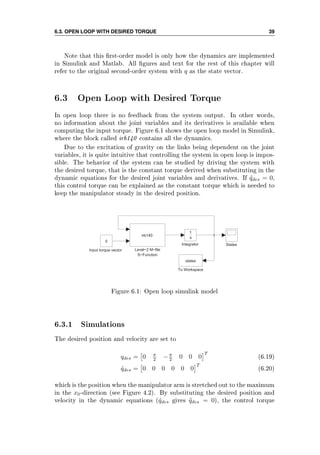
6.1 Open loop simulink model . . . . . . . . . . . . . . . . . . . . . . 39
6.2 Open loop response with desired torque, simulation 1 . . . . . . . 42
6.3 Open loop response with desired torque, simulation 2 . . . . . . . 42
6.4 Open loop response with desired torque, simulation 3 . . . . . . . 43
6.5 Open loop response with desired torque, simulation 4 . . . . . . . 43
6.6 Open loop response with zero torque, simulation 1 . . . . . . . . 47
6.7 Energy in the system with zero torque, simulation 1 . . . . . . . 47
6.8 Open loop response with zero torque, simulation 2 . . . . . . . . 48
6.9 Energy in the system with zero torque, simulation 2 . . . . . . . 48
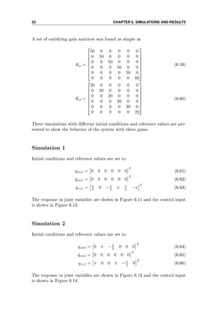
6.10 Closed loop simulink model with PD controllers . . . . . . . . . . 51
6.11 Closed loop position control response, simulation 1 . . . . . . . . 55
6.12 Closed loop position control input, simulation 1 . . . . . . . . . . 55
6.13 Closed loop position control response, simulation 2 . . . . . . . . 56
6.14 Closed loop position control input, simulation 2 . . . . . . . . . . 56
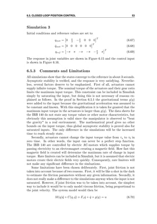
6.15 Closed loop position control response, simulation 3 . . . . . . . . 57
6.16 Closed loop position control input, simulation 3 . . . . . . . . . . 57
7.1 Conrming opposite q3-direction, simulation 1 . . . . . . . . . . . 60
7.2 Conrming opposite q3-direction, simulation 2 . . . . . . . . . . . 61
7.3 Euler-Lagrange closed loop position control response, simulation 1 63
7.4 Euler-Lagrange closed loop position control response, simulation 2 64
7.5 Euler-Lagrange closed loop position control response, simulation 3 64
vii

13. Chapter 1
Introduction
Robotics is concerned with the study of machines that can replace human beings.
The goal of this introductory chapter is to express the motivation behind the
thesis, and to give an overview of the contents. The IRB 140 is introduced,
as well as the objective and the software that has been used to solve it. An
outline and the contributions of the thesis is presented in the end of the chapter.
Historical facts are taken from [20] and [17].
1.1 History and Motivation
The English term robot was derived from the Czech word robota that means
executive labor, and was rst introduced by the Czech playwright Karel ƒapek
in his 1921 play Rossum's Universal Robots. Since then the term has been ap-
plied to virtually anything that operates with some degree of autonomy, usually
under computer control. An ocial denition of the term, dated to 1980, comes
from the Robot Institute of America (RIA) and reects todays status of robotics
technology:
A robot is a reprogrammable, multifunctional manipulator designed
to move material, parts, tools, or specialized devices through variable
programmed motions for the performance of a variety of tasks.
In the early 1980's, robot manipulators were touted as the ultimate solution
to automated manufacturing. Predictions were that entire factories of the future
would require few, if any, human operators. It turned out that these predictions
were a little exaggerated, as the savings in labor costs often did not outweigh
the development costs of creating robot systems. Quite simply, people are good
at what they do, and installing a robot involves complex systems integration
problems. As a result, robotics fell out of favor in the late 1980's.
A resurgence of interest in robotics can be witnessed in the recent years.
Deeper understanding of the subject and new technology have made it possi-
ble for robots to explore the surface on Mars, locate sunken ships, searching
1

14. 2 CHAPTER 1. INTRODUCTION
out land mines, and nding victims in collapsed buildings. In an industrial
environment the advantages of robots are reduction of manufacturing costs, in-
crease of productivity, improvement of quality standards, and the possibility of
eliminating harmful tasks for human operators.
1.2 The IRB 140
The IRB 140 (full name: IRB 140-6/0.8) is an industrial robot produced by
ABB, designed specically for manufacturing industries. Their website [14]
presents various facts about the manipulator, as well as articles, data sheets and
movies. The manipulator has a total of six revolute joints that are controlled by
AC-motors, hence six degrees of freedom (6 DOF). Figure 1.1 gives a clear view
of the manipulator and its degrees of freedom. The compact and robust design
is adapted for exible use, and the robot can be mounted on the oor, the wall
or the roof in any angle. It oers outstanding accuracy and speed, and suits
a lot of industrial tasks as for example spray painting, packing and palletizing.
The website presents some movies of the manipulator in work from companies
using it in their industry.
One of the data sheets on the website presents the Fanta Can Challenge.
This was a showcase from ABB to demonstrate the great accuracy of their mo-
tion control systems called QuickMove and TrueMove. The idea about Quick-
Move is to reach the end position in the shortest possible time, while TrueMove
ensures that the motion path followed is exactly the same independent of speed.
The latest experiment from 2009 involved three IRB 140 robots cooperating to
demonstrate the outstanding accuracy of the TrueMove concept. Movies from
the showcase are published on the website.
To achieve such accurate motion control, a complete dynamic model of the
robot is held in the robot controller. This model is considered a valuable trade
secret in ABB, and is not available even for buyers of the product. Dynamic pa-
rameters in their model are most likely estimated very thoroughly by numerous
days and months of measurements and tests with the manipulator. Dynamic
parameter identication is probably the greatest challenge in dynamic modeling
of robot manipulators, and will be highlighted in later chapters.
Discovering the Fanta Can Challenge as well as industrial areas of utilization
of the IRB 140 has denitely been a motivation for this thesis.
1.3 Objective
The objective of this thesis is to derive the complete dynamic model of the
IRB 140 by the Newton-Euler formulation. The work is a continuation of the
project work [6], where the dynamic model of the rst three degrees of freedom
of the manipulator were derived. All degrees of freedom are still modeled in
this thesis, and it should be mentioned that some denitions and parameters
ùsed in the project work are modied in this thesis to better suit the complete

15. 1.4. SOFTWARE 3
Figure 1.1: The IRB 140 with its six degrees of freedom [16]
model.
Dierent approaches on dynamic modeling of robot manipulators will be dis-
cussed, with particular focus on the Newton-Euler formulation. An automated
framework for deriving the dynamic model by the Newton-Euler formulation will
be presented, and this framework will then be utilized for the IRB 140. Param-
eters will be dened by searching for applicable information in the manipulator
data sheets, as well as by parameter estimation when required. Limitations in
the dynamic model will be described to underline how it diers from a perfect
model.
The model will be studied in open loop and closed loop to investigate stabil-
ity and energy properties. Based on a Lyapunov stability analysis, a mathemat-
ical proof of global asymptotic stability for position control will be presented.
Then the model for the IRB 140 will be simulated in closed loop to verify this
mathematical proof.
Ultimately, some results will be compared to the results of an equivalent
dynamic model derived by the Euler-Lagrange formulation [13].
1.4 Software
Three computer programs have been used to solve the thesis assignment. Fol-
lowing is a short description of this software and the area of utilization.

16. 4 CHAPTER 1. INTRODUCTION
Maple 15
Maple [9] is developed by MapleSoft, and is a technical computing software
for doing symbolic, numeric and graphical computations. Because of its great
eciency in symbolic computations, Maple has been used to derive the dynamic
model for the IRB 140. The framework for deriving dynamic models of any serial
robot manipulator with revolute joints has been designed in Maple as well.
Matlab R2010a with Simulink 7.5
Matlab [10] is developed by MathWorks, and is a high-level language and nu-
merical computing environment for performing computationally intensive tasks
faster than with traditional programming languages. It oers tight integration
with other MathWorks products, among them Simulink [11] which is an en-
vironment for multidomain simulation and Model-Based Design for dynamic
and embedded systems. Matlab and Simulink have been used to simulate the
dynamic model for the IRB 140, and to present the results graphically.
Adobe Illustrator CS4
Adobe Illustrator [21] is a vector graphics editor developed by Adobe Systems.
It oers sophisticated drawing tools with high precision that is intuitively easy
to use. Most gures in this thesis are designed with this software.
1.5 Outline
• Chapter 2: Fundamental background theory and notation used through-
out the thesis are explained in this chapter. It is put importance on the
standard convention of how to interpret robot manipulators, as well as
the concept of rotation matrices.
• Chapter 3: This chapter presents dierent approaches on dynamic mod-
eling of robot manipulators, and compares the Newton-Euler formulation
to the Euler-Lagrange formulation. The derivation of the Newton-Euler
formulation is followed in detail, and an automated framework for dynamic
modeling using this formulation is presented.
• Chapter 4: It is shown how the IRB 140 is interpreted as a kinematic
chain following the standard convention. Parameters of the system is
dened on the basis of information from the manipulator data sheets and
parameter estimation.
• Chapter 5: The Newton-Euler formulation is applied on the IRB 140,
and the forward and backward recursions are followed for all links in the
kinematic chain.

17. 1.6. CONTRIBUTIONS 5
• Chapter 6: This chapter presents simulations of the system in open loop
and closed loop. The results include energy investigations and stability
analyses, where simulations in closed loop with PD controllers veries a
remarkable mathematical proof.
• Chapter 7: It is presented a comparison of some of the results from this
thesis, with the results of the dynamic model of the same manipulator by
the standard Euler-Lagrange formulation.
• Chapter 8: This chapter presents the concluding summary of the thesis,
as well as recommendations for future work.
1.6 Contributions
• A complete derivation of the Newton-Euler formulation in general. The
derivation is based on the one in [20], but is corrected and restated due
to the discoveries of misleading notations and errata in the book (see
Appendix D).
• An automated framework for deriving the dynamic model of any serial
robot manipulator with rigid links and revolute joints. It can easily be
adjusted to any number of degrees of freedom, and if desired, it is not a
comprehensive task to modify it for prismatic joints as well.
• A convenient representation of the IRB 140 as a kinematic chain of sin-
gle degree-of-freedom joints. The way the frames are attached leads to
signicant simplications in the derivation of the dynamic model by the
Newton-Euler formulation.
• The complete dynamic model of the IRB 140, including simulations that
demonstrate satisfying behavior of the model in open loop and closed loop.
The framework used is designed in such a way that all parameters can be
easily modied.
• An investigation of eciency when using the Newton-Euler formulation
and the Euler-Lagrange formulation to derive the dynamic model for the
IRB 140. The results show a clear advantage of utilizing a recursive pro-
cedure for such a complex system.

19. Chapter 2
Background Theory and
Notation
This thesis follows the standard convention of how a robot manipulator is in-
terpreted. Fundamental background theory and important notation that are
used throughout the thesis are briey explained in this chapter to facilitate the
understanding of the later chapters.
Understanding the concept of rotation matrices is an essential part of mod-
eling robot manipulators. Section 2.1 describes rotational transformations and
presents some important properties of rotation matrices and their relation to
skew symmetric matrices. Section 2.2 shows how a robot manipulator is com-
posed by links and joints to form a kinematic chain, and presents guidelines of
how to dene the links, joints and frames. The material is mainly taken from
[20].
The rest of the chapter is dedicated to the concepts of feedback controllers,
the inertia tensor, and positive and negative deniteness. A complete descrip-
tion of these concepts are given in most books about control theory, e.g. [3], [8]
and [20].
2.1 The Rotation Matrix
In order to perform algebraic manipulations with vectors using coordinates, it is
essential that all vectors are expressed in the same coordinate frame. Rotation
matrices are used to accomplish this. An n×n rotation matrix species the ori-
entation of one frame relative to another frame in the n-dimensional Euclidean
space. To specify the coordinate vectors of frame 1 with respect to frame 0 in
three dimensions, the 3 × 3 rotation matrix is written as
R0
1 = x0
1 y0
1 z0
1 (2.1)
where the columns are the coordinates of the vectors x1, y1, and z1 expressed
in frame 0.
7

20. 8 CHAPTER 2. BACKGROUND THEORY AND NOTATION
2.1.1 Vectors and Rotational Transformations
A vector species a direction and a magnitude in the Euclidean space, and can be
assigned coordinates with respect to a reference coordinate frame. That means
a particular vector is always the same geometric entity, but the representation of
the vector by coordinates depends directly on the reference coordinate frame.
So that the reference frame will always be clear, vectors are denoted with a
superscript to show in which frame they are expressed. Introducing two frames
(frame 0 and frame 1) and a vector v, that means v0
is v expressed in frame
0, while v1
is v expressed in frame 1. Introducing a third frame (frame 2), the
relationship between the vector v and the frames becomes
v0
= R0
1v1
(2.2)
v1
= R1
2v2
(2.3)
v0
= R0
2v2
(2.4)
which gives
R0
2 = R0
1R1
2 (2.5)
2.1.2 Properties of the Rotation Matrices
In a coordinate frame, the axes are always dened as unit vectors that are
mutually orthogonal. A rotation matrix species the relationship between two
such frames, and is therefore also said to be orthogonal. Restricting all coordi-
nate frames to be right handed frames, such rotation matrices are denoted as
the Special Orthogonal group of order n, shortened as SO(n), where n is the
number of dimensions. Any rotation matrix R ∈ SO(n) has some important
properties, and they are
• RT
= R−1
∈ SO(n)
• The columns (and therefore the rows) of R are mutually orthogonal
• Each column (and therefore each row) of R is a unit vector
• det R = 1
2.1.3 Relation to Skew Symmetric Matrices
An n × n matrix S is said to be skew symmetric if and only if
ST
+ S = 0 (2.6)
which means that every 3 × 3 skew symmetric matrix has the form
S =


0 −s3 −s2
s3 0 −s1
−s2 s1 0

 (2.7)
Skew symmetric matrices have been found useful in relation to rotation
matrices. Four important properties are given below.

21. 2.2. KINEMATIC CHAINS 9
1. For any vectors a and p belonging to R3
,
S(a)p = a × p (2.8)
where S is a 3×3 skew symmetric matrix.
2. For R ∈ SO(3) and a ∈ R3
RS(a)RT
= S(Ra) (2.9)
where S is a 3×3 skew symmetric matrix.
3. In the general case of angular velocity about an arbitrary and possibly
moving axis we have
˙R(t) = S(ω(t))R(t) (2.10)
where R = R(t) ∈ SO(3) for every t ∈ R, S is a 3×3 skew symmetric
matrix, and ω(t) is the angular velocity of the rotating frame with respect
to the xed frame at time t.
4. For an n × n skew symmetric matrix S and any vector X ∈ Rn
XT
SX = 0 (2.11)
2.2 Kinematic Chains
Robot manipulators are composed of links connected by joints to form a kine-
matic chain, where the joints are revolute or prismatic. A revolute joint is like
a hinge and allows relative rotation between two links, while a prismatic joint
allows a linear relative motion between two links. Both types of joints have a
single degree of freedom, thus each joint i can be represented by a single joint
variable qi. Figure 2.1 shows a symbolic representation of robot joints in 2D
and 3D.
Figure 2.1: Symbolic representation of robot joints [20]
A conguration of a manipulator is a complete specication of every point
on the manipulator. Assuming a manipulator with rigid links and a xed base,

22. 10 CHAPTER 2. BACKGROUND THEORY AND NOTATION
that means the conguration is entirely given by q, the vector of joint variables.
In case of joints with more degrees of freedom, like a ball or a spherical wrist,
these joints can always be thought of as a succession of joints with a single
degree of freedom.
A coordinate frame is rigidly attached to each link, and an inertial frame is
attached to the robots base. Links, joints and frames are dened as summarized
below.
• Links are numbered from 0 to n where link 0 is the base.
• Joints are numbered from 1 to n where joint i connects link i − 1 to link
i.
• When joint i is actuated, link i moves. The base can not be actuated.
• Frames are numbered from 0 to n where frame i is attached to link i.
• Frames are attached such that axis zi of frame i is the axis of actuation
for joint i + 1.
• The joint variable qi is associated with joint i.
As an example, Figure 2.2 shows these denitions applied in the case of an
elbow manipulator with three degrees of freedom.
BASE
x₀
Link 1
y₀z₀
q₁
y₁
z₁
x₁
q₂
y₂
z₂
q₃
x₂
y₃
x₃
z₃
Link 2 Link 3
Joint 1
Joint 2 Joint 3
Figure 2.2: Links, joints and coordinate frames on an elbow manipulator

23. 2.3. THE INERTIA TENSOR 11
2.3 The Inertia Tensor
The moment of inertia is a scalar value expressing the resistance to changes to
the rotation of an object. If the axis of rotation is not given, it is possible to
generalize the scalar moment of inertia to a 3×3 matrix expressing the moment
of inertia about arbitrary axes. This matrix is called the inertia tensor.
Let the mass density of an object be represented as a function of position,
ρ(z, y, z). Then the inertia tensor in a frame attached to the center of mass of
the object is computed as
I =


Ixx Ixy Ixz
Iyx Iyy Iyz
Izx Izy Izz

 (2.12)
where
Ixx = (y2
+ z2
)ρ(x, y, z)dx dy dz (2.13)
Iyy = (x2
+ z2
)ρ(x, y, z)dx dy dz (2.14)
Izz = (x2
+ y2
)ρ(x, y, z)dx dy dz (2.15)
and
Ixy = Iyx = − xyρ(x, y, z)dx dy dz (2.16)
Ixz = Izx = − xzρ(x, y, z)dx dy dz (2.17)
Iyz = Izy = − yzρ(x, y, z)dx dy dz (2.18)
The diagonal elements Ixx, Iyy, Izz are called the principal moments of inertia,
and the o-diagonal terms are called the cross products of inertia. If the mass
distribution of the object is symmetric with respect to the attached frame, then
the inertia tensor will be diagonal (cross products of inertia are identically zero).
2.4 Feedback Controllers
A system can be controlled in open loop or closed loop. With an open-loop
controller, the input is computed without observing the output that it is con-
trolling. Complex systems will not be possible to control in open loop, because
the controller will never know if the output has achieved the desired goal. How-
ever, by adding feedback controllers, it might be possible to stabilize the system
in closed loop.
A feedback controller observes the output and calculates the error between
this output and a reference value. Then the input is computed based on this

24. 12 CHAPTER 2. BACKGROUND THEORY AND NOTATION
error such that the output approaches the reference value. To achieve a desired
behavior of the output, controllers can take one or more of three standard
control elements. These elements are
• P - proportional term: The input is proportional to the error between
the reference value and the current output. Kp is the proportional gain.
• I - integral term: Integrates the error over time and multiplies with the
integral gain Ki. The term eliminates steady state error.
• D - derivative term: Determines the slope of the error over time and
multiplies with the derivative gain Kd. The term has as a damping eect.
2.5 Positive and Negative Deniteness
A function V (x) satisfying the conditions V (0) = 0 and V (x) 0 for x = 0
is said to be positive denite. If it satises V (0) = 0 and the weaker second
condition V (x) ≥ 0 for x = 0 it is said to be positive semidenite. The function
V (x) is said to be negative denite if −V (x) is positive denite, and negative
semidenite if −V (x) is positive semidenite.
Functions of the quadratic form
V (x) = xT
Px (2.19)
where P is a real symmetric matrix, can easily be checked for sign deniteness
by inspecting P. If all eigenvalues of P are positive (nonnegative), which is true
if and only if all the leading principal minors of P are positive (nonnegative),
then V (x) is a positive denite (positive semidenite) function. If V (x) is a
positive denite (positive semidenite) function, the matrix P is also said to
be positive denite (positive semidenite). Finally, P is said to be negative
denite if −P is positive denite, and negative semidenite if −P is positive
semidenite.
It is common practice to write P 0 if P is positive denite, and P ≥ 0 if
P is positive semidenite.

25. Chapter 3
Dynamic Modeling of Robot
Manipulators in General
Robot manipulators can be described mathematically in dierent ways. The
problem of kinematics is to describe the motion of the manipulator without
consideration of forces and torques causing the motion. These equations de-
termine the position and orientation of the end eector given the values for
the joint variables (forward kinematics), and as the opposite the values of the
joint variables given the position and orientation of the end eector (inverse
kinematics).
Dynamic modeling means deriving equations that explicitly describes the re-
lationship between force and motion. These equations are important to consider
in simulation of robot motion, and in design of control algorithms. The most
important concepts in fundamental robotics including kinematics, dynamics and
control are given in [20] and [17].
Section 3.1 deals with dierent approaches on dynamic modeling of robot
manipulators. The Euler-Lagrange formulation and the Newton-Euler formu-
lation are introduced, and techniques for dynamic parameter estimation are
briey described.
General equations of the Newton-Euler formulation are derived in detail in
Section 3.2. The whole derivation from the basis of mechanic laws to the nal
equations of n-link manipulators is followed in detail. The chapter ends by
presenting an automated framework for deriving the dynamic manipulator of
any serial robot manipulator with revolute joints.
3.1 Dierent Approaches
Computing the dynamics of robot manipulators can be challenging. Researchers
have discovered dierent approaches, where in general there are two methods
available; the Euler-Lagrange formulation and the Newton-Euler formulation.
In the standard Euler-Lagrange formulation the manipulator is treated as a
13

26. 14 CHAPTER 3. DYNAMIC MODELING OF ROBOT MANIPULATORS IN GENERAL
whole, and the system is analyzed based on its kinetic and potential energy. The
Newton-Euler formulation is quite dierent because each link of the manipulator
is treated in turn. First there is a forward recursion describing its linear and
angular motion, then a backward recursion to calculate the forces and torques.
Both of these formulations are derived from rst principles in [20] and [17],
including examples of how the methods can be applied. The resulting dynamic
model is the same for both methods and can be written in matrix form as
M(q)¨q + C(q, ˙q) ˙q + g(q) = u (3.1)
where
q = vector of joint variables
u = vector of torques
M = inertia matrix
C = centrifugal and Coriolis terms
g = gravity vector
3.1.1 Euler-Lagrange versus Newton-Euler
The eciency of the Euler-Lagrange formulation and the Newton-Euler formu-
lation is an interesting topic. Actually there is no clear answer to the question of
which method is better than the other. The main goal is to derive the dynamic
model as fast as possible, and how well this goal is satised for each method de-
pends on several factors. The number of link and joints in the kinematic chain,
the topology of the chain (e.g. serial or parallel), the position and orientation
of the coordinate frames, and whether a recursive procedure is used or not, are
factors that will inuence the computation time.
The Newton-Euler formulation is usually the preferred choice for manipula-
tors with many degrees of freedom. The reason is the recursive structure which
the Newton-Euler formulation is based on. If the frames are attached in a con-
venient way (see Section 5.1), the recursions will be greatly simplied. This
advantage of the Newton-Euler formulation is supported in [7] which proves
that a recursive approach is in general faster than treating the manipulator as
a whole. It should also be mentioned that for the case of parallel manipulators,
it is shown in [5] that the Newton-Euler formulation gives an advantage for
dynamic computations and control.
However, [7] shows that it is also possible to compute the Euler-Lagrange
formulation in a recursive procedure, and [19] shows that the computation time
of the two algorithms are equivalent if the frames are attached optimally in both
formulations.
In the end, the choice of algorithm is a matter of personal preference, and
the main reason for choosing one method over the other is that it might provide
dierent insights. An interesting detail is discovered and explained in Chapter
5, when the Newton-Euler formulation is applied on the IRB 140.

27. 3.2. DERIVATION OF THE NEWTON-EULER FORMULATION 15
3.1.2 Dynamic Parameter Identication
Using the dynamic model (3.1) for solving simulation and control problems
demands the knowledge of values of dynamic parameters of the manipulator.
In general, a given rigid body is described by ten such parameters; the mass,
the six independent entries of the inertia tensor, and the three coordinates of
the center of mass. However, due to constraints and coupled kinematics, this
number could be lower for a manipulator. An n-link robot then has a maximum
of 10n dynamic parameters. Estimating the parameters from the design data
of the manipulator is not simple, but there are a few techniques available.
In order to nd accurate estimates of the dynamic parameters, it is possible
to use an identication technique which exploits that the dynamic model are
linear with respect to a suitable set of dynamic parameters. The system (3.1)
can be written as
M(q)¨q + C(q, ˙q) ˙q + g(q) = Y (q, ˙q, ¨q)Θ (3.2)
where Y (q, ˙q, ¨q) is called the regressor and Θ is the parameter vector. Assum-
ing that values of the joint positions q, velocities ˙q, and accelerations ¨q can be
recorded during execution of trajectories with the manipulator, and that the
joint torques can be measured from sensors in the joints or current measure-
ments, it is now possible to calculate the dynamic parameters directly by the
parameterized system (3.2). However, nding a minimal set of parameters that
can parametrize the dynamic model is dicult in general, and as mentioned,
measurements of q, ˙q, ¨q during motion is a requirement for using this method.
Another approach is Computer-Aided-Design (CAD) modeling. The various
components of the manipulator are then modeled digitally on the basis of their
geometry and type of materials, and features in the CAD system can be used to
measure the parameters. Inaccuracies will occur with this technique, because
of simplications in the modeling and the loss of information about complex
dynamic eects like joint friction.
Dynamic parameter identication is explained more detailed in [20] and [17].
3.2 Derivation of the Newton-Euler Formulation
The rest of this chapter is dedicated to derive equations of the Newton-Euler
formulation to be applied on the IRB 140. Section 3.2.1 describes the gen-
eral case based on important mechanic laws, while Section 3.2.2 modies the
equations to suit any serial n-link manipulator with revolute joints.
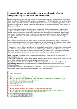
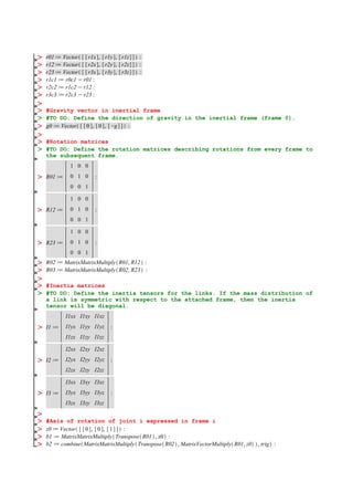
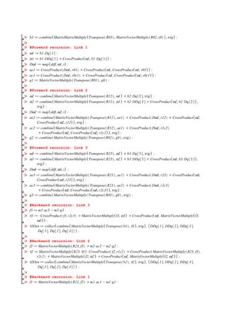
Section 3.2.3 presents a framework for deriving the dynamic model of any
serial robot manipulator with only revolute joints. The framework is designed
in Maple and can be found in the attached ZIP-le, in addition to the printed
version showed in Appendix B.
The following derivation of the Newton-Euler formulation is entirely based
on the derivation presented in [20]. The reason for restating all the details is
that there was discovered several misleading notations and errata in the book.
Appendix D presents a list of these ndings.

28. 16 CHAPTER 3. DYNAMIC MODELING OF ROBOT MANIPULATORS IN GENERAL
3.2.1 The General Case
The basis of the Newton-Euler formulation is three important mechanic laws:
• Every action has an equal and opposite reaction. Thus, if link 1 applies a
force f and torque τ to link 2, then link 2 applies a force −f and torque
−τ to link 1.
• The rate of change of the linear momentum equals the total force applied
to the link.
• The rate of change of the angular momentum equals the total torque
applied to the link.
Applying the second law to the linear motion of a link gives the relationship
d(mv)
dt
= f (3.3)
where m is the mass of the link, v is the velocity of the center of mass with
respect to an inertial frame, and f is the sum of external forces applied to the
link. Since the mass is constant as a function of time for robot manipulators,
Equation (3.3) can be simplied to
f = ma (3.4)
where a is the acceleration of the center of mass.
The third law gives the relationship
d(I0ω0)
dt
= τ0 (3.5)
where I0 is the moment of inertia of the link, ω0 is the angular velocity of the
link, and τ0 is the sum of torques applied on the link. All three variables are
expressed in an inertial frame whose origin is at the center of mass. Note that
I0 is not necessarily a constant function of time, but this can be taken care of
by rewriting Equation (3.5) to be valid for a frame rigidly attached to the the
link instead of an inertial frame. A similarity transformation of I0 is given by
I = R−1
I0R (3.6)
which gives
I0 = RIRT
(3.7)
where R is the rotation matrix that transforms coordinates from the link at-
tached frame to the inertial frame. Equation (3.7) together with the facts
ω0 = Rω, τ0 = Rτ (3.8)

29. 3.2. DERIVATION OF THE NEWTON-EULER FORMULATION 17
yields
d(I0ω0)
dt
=
d(RIRT
Rω)
dt
(3.9)
=
d(RIω)
dt
(3.10)
= ˙RIω + RI ˙ω (3.11)
and the equation for the rate of change of the angular momentum with respect
to the link attached frame is
τ = RT
τ0 (3.12)
= RT
( ˙RIω + RI ˙ω) (3.13)
= RT ˙RIω + I ˙ω (3.14)
The rotation matrix in Equation (3.14) can be cancelled out by taking advantage
of the properties (2.8), (2.9) and (2.10). The nal torque expression becomes
τ = RT ˙RIω + I ˙ω (3.15)
= RT
S(ω0)RIω + I ˙ω (3.16)
= S(RT
ω0)Iω + I ˙ω (3.17)
= S(ω)Iω + I ˙ω (3.18)
= ω × (Iω) + I ˙ω (3.19)
This concludes the general case of the derivation with the force balance and
moment balance summarized respectively as
f = ma (3.20)
τ = ω × (Iω) + I ˙ω (3.21)
3.2.2 Equations of an n-link Manipulator
To begin with, several vectors need to be introduced. Note that all these vectors
are expressed in frame i.

30. 18 CHAPTER 3. DYNAMIC MODELING OF ROBOT MANIPULATORS IN GENERAL
ac,i = acceleration of the center of mass of link i
ae,i = acceleration of the end of link i (origin of frame i + 1)
ωi = angular velocity of frame i with respect to frame 0
αi = angular acceleration of frame i with respect to frame 0
zi = axis of actuation of frame i with respect to frame 0
gi = acceleration due to gravity
fi = force exerted by link i − 1 on link i
τi = torque exerted by link i − 1 on link i
Ri
i+1 = rotation matrix from frame i to frame i + 1
mi = the mass of link i
Ii = inertia tensor of link i about a frame parallel to frame i
whose origin is at the center of mass of link i
ri−1,ci = vector from the origin of frame i − 1 to the center of mass of link i
ri−1,i = vector from the origin of frame i − 1 to the origin of frame i
ri,ci = vector from the origin of frame i to the center of mass of link i
−1, ,
− +1 +1
− +1 +1
Figure 3.1: Forces and torques acting on a random link
Figure 3.1 shows a random link together with all forces and torques acting on it.
By the law of action and reaction, fi is the force exerted by link i − 1 on link i,
and −fi+1 is the force exerted by link i+1 on link i. According to the denitions
above, fi is expressed in frame i while −fi+1 is expressed in frame i + 1, thus
to express both forces in frame i it is required to multiply the latter with Ri
i+1.
The same apply to the torque, again by the law of action and reaction.
When all vectors in Figure 3.1 are expressed in frame i, the force balance
equation based on (3.20) can be stated as
link
f = ma (3.22)
fi − Ri
i+1fi+1 + migi = miac,i (3.23)
fi = Ri
i+1fi+1 + miac,i − migi (3.24)
Next, the moment balance equation for the link will be computed, and it is
important to note two things. First, the moment exerted by a force f about a
point is given by f × r, where r is the radial vector from the point where the
force is applied to the point where the moment is computed. Second, the vector

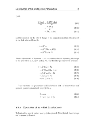
31. 3.2. DERIVATION OF THE NEWTON-EULER FORMULATION 19
migi does not appear in the moment balance since it is applied directly at the
center of mass. The moment balance equation based on (3.21) becomes
link
τ = ω × (Iω) + I ˙ω (3.25)
τi − Ri
i+1τi+1 + fi × ri−1,ci − (Ri
i+1fi+1) × ri,ci = ωi × (Iiωi) + Iiαi (3.26)
τi = Ri
i+1τi+1 − fi × ri−1,ci + (Ri
i+1fi+1) × ri,ci + ωi × (Iiωi) + Iiαi (3.27)
The force balance equation is actually a part of the moment balance equation.
Solving Equation (3.27) for decreasing i and substituting (3.24) is the ultimate
goal of the formulation, but the solution needs to be expressed only by q, ˙q, ¨q
and constant parameters to achieve the general matrix form (3.1). That means
it is necessary to nd a relation between q, ˙q, ¨q and ac,i, ωi and αi. This can
be obtained by a recursive procedure of increasing i.
Since the force and moment equations are expressed with respect to the link
attached frame, this also applies to ac,i, ωi and αi. However, as a starting point,
ωi and αi need to be expressed in the inertial frame, and the superscript (0)
will be used to denote that. This gives
ω
(0)
i = ω
(0)
i−1 + zi−1 ˙qi (3.28)
because of the fact that the angular velocity of frame i equals that of frame i−1
plus the added rotation from joint i. Using rotation matrices this leads to
ωi = (Ri−1
i )T
ωi−1 + bi ˙qi (3.29)
where
bi = (R0
i )T
R0
i−1z0 (3.30)
is the rotation of joint i expressed in frame i.
For the angular acceleration it is important to note that
αi = (R0
i )T
˙ω
(0)
i (3.31)
which means αi = ˙ωi! By using Newtons Second Law in a rotating frame (see
[22], page 342-343), the time derivative of Equation (3.28) becomes
˙ω
(0)
i = ˙ω
(0)
i−1 + zi−1 ¨qi + ω
(0)
i × zi−1 ˙qi (3.32)
and expressed in frame i it directly becomes
αi = (Ri−1
i )T
αi−1 + bi ¨qi + ωi × bi ˙qi (3.33)
Now it only remains to nd an expression for ac,i. First, the linear velocity
of the center of mass of link i is expressed as
v
(0)
c,i = v
(0)
e,i−1 + ω
(0)
i × r
(0)
i−1,ci (3.34)

32. 20 CHAPTER 3. DYNAMIC MODELING OF ROBOT MANIPULATORS IN GENERAL
and note that r
(0)
i−1,ci is constant in frame i. Thus
a
(0)
c,i = a
(0)
e,i−1 × r
(0)
i−1,ci + ω
(0)
i × (ω
(0)
i × r
(0)
i−1,ci) (3.35)
Multiplying with rotation matrices and using the fact that
R(a × b) = (Ra) × (Rb) (3.36)
the nal expression for the acceleration of the center of mass of link i, expressed
in frame i, becomes
ac,i = (Ri−1
i )T
ae,i−1 + ˙ωi × ri−1,ci + ωi × (ωi × ri−1,ci) (3.37)
To nd the acceleration of the end of the link, ri−1,ci is replaced by ri−1,i
ae,i = (Ri−1
i )T
ae,i−1 + ˙ωi × ri−1,i + ωi × (ωi × ri−1,i) (3.38)
This completes the recursive formulation, and the Newton-Euler formulation
of an n-link manipulator can be stated as follows.
1. Forward recursion: Start with the initial conditions
ω0 = α0 = ac,0 = ae,0 = 0 (3.39)
and solve Equations (3.29), (3.33), (3.38) and (3.37) (in that order) to
compute ωi, αi and ac,i for increasing i from 1 to n.
2. Backward recursion: Start with the terminal conditions
fn+1 = τn+1 = 0 (3.40)
and solve Equations (3.24) and (3.27) (in that order) for decreasing i from
n to 1.
3.2.3 Automated Framework
This section introduces an automated framework for deriving the dynamic
model of robot manipulators by the Newton-Euler formulation. The frame-
work is given in printed form in Appendix B, and the digital le can be found
in the attached ZIP-le. The dynamic model of the IRB 140 is derived by this
framework.
The framework is restricted to manipulators with rigid links and only revo-
lute joints, but it can be adjusted to suit other kinds of manipulators if desired.
The composition presented is for three degrees of freedom, but due to the recur-
sive procedure it can easily be adjusted to any number of degrees of freedom.
Complex manipulators with several degrees of freedom will result in huge
dynamic systems, and it might be desirable to evaluate smaller parts of a system
individually. Every element of the inertia matrix, as well as the gravity compo-
nents and the Coriolis and centrifugal components, are evaluated individually
towards the end of the framework.

33. 3.2. DERIVATION OF THE NEWTON-EULER FORMULATION 21
The Matlab conversion code used in the end can be applied to any expression,
and is a simple way to convert Maple code to Matlab code. Note that the
joint variable derivatives are not known in the Matlab conversion code. These
quantities will have to be redened as desired in Matlab.
It is optional to dene symbolic values if the goal is a less specic model,
but note that the more symbolic values and the less dened zeros, the larger
dynamic model.
All quantities must be dened according to the denitions and notation
introduced in Section 3.2.2. In addition, it is important to add or remove lines
following the recursive procedure, according to the how many degrees of freedom
there are in the manipulator to be analyzed. A look at the Maple code for the
IRB 140 with six degrees of freedom will clarify these adjustments (Appendix
C).
Explanations for the parts that has to be adjusted are given below. These
parts are grayed out in the framework.
• Joint variables: Specify the number of joint variables (degrees of free-
dom) in the manipulator by adjusting the q-vector.
• Link length vectors and vectors to the centers of mass: Dene
the link length vectors and the vectors to the centers of mass, which all
are independent of conguration.
• Gravity vector in inertial frame: Dene the direction of gravity in
the inertial frame (frame 0).
• Rotation matrices: Dene the rotation matrices describing rotations
from every frame to the subsequent frame.
• Inertia matrices: Dene the inertia tensors for the links. If the mass
distribution of a link is symmetric with respect to the attached frame,
then the inertia tensor will be diagonal.

35. Chapter 4
System Description and
Dynamic Parameter
Estimation
ABB has produced the industrial robot manipulator named IRB 140. Their
website [14] presents facts about the manipulator, as well as articles and movies
from experiments and from companies using the manipulator.
This chapter is presenting all information about the IRB 140 which is needed
to derive the dynamic model by the Newton-Euler formulation. The manipula-
tor comes with a product manual, a product specication [16], and a data sheet
(Appendix A and [15]). The manual is not of much interest in this thesis, as
it focuses solely on safety, installation and maintenance. What is interesting
is the data sheet, which is basically a summary of the product specication,
presenting some facts about the structure and performance of the manipulator.
The relevant information given in the data sheets are summarized in Section
4.1.
Out of consideration for trade secrets in ABB, the data sheets present a very
limited amount of information. Section 4.2 states the these limitations and how
they lead to simplied dynamic parameter estimation.
In Section 4.3, a symbolic representation shows how the joints and links
can be represented as a serial kinematic chain, and how frames are attached to
the links. This representation follows all guidelines described in the previous
chapters, and can be said to lay the foundation for the whole dynamic model.
Parameter estimation is carried out in Section 4.4.
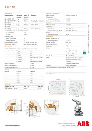
4.1 Information from Data Sheets
As mentioned in Section 1.2, the manipulator has a total of six revolute joints
that are controlled by AC-motors, hence six degrees of freedom (6 DOF). The
23

36. 24 CHAPTER 4. SYSTEM DESCRIPTION AND DYNAMIC PARAMETER ESTIMATION
total mass including the base and without a payload is 98 kg, and the mass of
the payload alone must not exceed 6 kg. Some applicable link dimensions are
given in Figure 4.1 (lengths in millimeters).
(a) View of the manipulator
from the back
(b) View of the manipulator from the side
Figure 4.1: View of the manipulator from the back and side [16]
4.2 Limitations
It is not possible to derive an accurate dynamic model for the IRB 140 with
the limited information available in the data sheets. No dynamic parameters
for the links are given, and as explained in Section 3.1, these parameters are
indeed a demanding task to estimate. The masses of the links could have been
identied by dismantling the manipulator and weigh them one by one, but this
would have been a comprehensive task by itself. Besides, doing this would not
come in particularly useful anyway, unless thorough experiments on estimating
the inertia parameters and centers of mass were to be performed as well.
Performing dynamic parameter identication of the IRB 140 is an interest-
ing and challenging task, but would require the possibility to measure q, ˙q, ¨q,
or knowledge about alternative identication methods like for example CAD
modeling (would again require detailed information about the shape and mate-
rials of the manipulator). ABB does not give their customers access to measure

37. 4.3. MODELING SET-UP 25
the states of the robot manipulators, not even access to the controller parame-
ters. Consequently, the dynamic parameters in the model have been estimated
quite roughly. The estimation is based on intuitive guesses, with the purpose of
creating a simple model which still represents the IRB 140 as good as possible.
4.3 Modeling Set-up
The IRB 140 can be interpreted in such a way that the rst three degrees of
freedom make up an elbow manipulator, and the last three degrees of freedom
is a spherical wrist attached to the end of the arm. This spherical wrist alone
is built up by three single degree-of-freedom revolute joints, where the rotation
axes intersect in the wrist center point. Thus the two links in between will have
zero length and zero mass.
Examining the manipulator closer, it is discovered that some freedom is
given to the choice of how to model joint 4. Actually, modeling the last three
joints as a spherical wrist is not the desired choice, because the two links in
between (link 4 and 5) do not have zero length and mass. To compensate for
this, it is found convenient to interpret the manipulator such that joint 3 and
4 has their center point in common, and joint 5 and 6 has their center point in
common. In that case it is link 3 and link 5 which is modeled with zero length
and mass. Figure 4.2 shows a symbolic representation of the manipulator by
this interpretation, including how the frames have been attached to the links.
BASE
x₀
y₀
z₀
q₁
y₁
x₁
z₁
q₂
q₃
y₃
x₂,x₃
z₂
y₂,z₃
q₄
q₅
x₅
x₄
z₄,y₅
y₄,z₅
q₆
x₆
z₆
y₆
Figure 4.2: Symbolic representation of the IRB 140

38. 26 CHAPTER 4. SYSTEM DESCRIPTION AND DYNAMIC PARAMETER ESTIMATION
All rotation matrices can be calculated as products of basic rotations about
the z-axis and the x-axis, where these basic rotation matrices are dened in
general form as
Rz,θ =


cos(θ) −sin(θ) 0
sin(θ) cos(θ) 0
0 0 1

 , Rx,θ =


1 0 0
0 cos(θ) −sin(θ)
0 sin(θ) cos(θ)

 (4.1)
where θ is the rotation angle. Observing Figure 4.2, it is quite straight forward
to calculate rotation matrices for the manipulator by substituting q and the
constant rotations for θ. Note the simplications due to all constant rotations
being multiples of π
2 . The result becomes
R0
1 =


cos(q1) 0 −sin(q1)
sin(q1) 0 cos(q1)
0 −1 0

 (4.2)
R1
2 =


cos(q2 − π
2 ) −sin(q2 − π
2 ) 0
sin(q2 − π
2 ) cos(q2 − π
2 ) 0
0 0 1

 (4.3)
R2
3 =


cos(q3) 0 −sin(q3)
sin(q3) 0 cos(q3)
0 −1 0

 (4.4)
R3
4 =


cos(q4) 0 sin(q4)
sin(q4) 0 −cos(q4)
0 1 0

 (4.5)
R4
5 =


cos(q5 + π) 0 sin(q5 + π)
sin(q5 + π) 0 −cos(q5 + π)
0 1 0

 (4.6)
R5
6 =


cos(q6) −sin(q6) 0
sin(q6) cos(q6) 0
0 0 1

 (4.7)
Further multiplications by a recursive procedure yield
R0
2 = R0
1R1
2 (4.8)
R0
3 = R0
2R2
3 (4.9)
R0
4 = R0
3R3
4 (4.10)
R0
5 = R0
4R4
5 (4.11)
R0
6 = R0
5R5
6 (4.12)
4.4 Parameter Estimation
This section describes how the dynamic parameters are estimated. It is men-
tioned in Section 4.2 that the parameters are estimated quite roughly. Still they

39. 4.4. PARAMETER ESTIMATION 27
should be close enough to the real unknown parameters that simulations show
a behavior that is somewhat in accordance to the behavior of a perfect model.
The centers of mass of the four links have been estimated by studying the
manipulator thoroughly, assuming the links have uniform mass density. Figure
4.3 shows the estimated centers of mass with colored dots. Link 1 has a red dot,
link 2 has a green dot, link 4 has a blue dot, and link 6 has a yellow dot. Note
that viewing from the back in Figure 4.3(a), link 4 and 6 have their centers of
mass along the same line perpendicular to the paper.
(a) The centers of mass
from the back
(b) The centers of mass from the side
Figure 4.3: The centers of mass from the back and side [16]
Vectors between the origins of the frames are dened precisely by the dimen-
sions in Figure 4.3. Vectors from the origins of the frames to the centers of mass
are calculated by rst computing the scale of the gure, and then multiplying
the scale with the lengths measured by a ruler. The clever way of attaching
frames to the links in the Newton-Euler formulation make all length vectors in-
dependent of the conguration of the manipulator. The results are given below

40. 28 CHAPTER 4. SYSTEM DESCRIPTION AND DYNAMIC PARAMETER ESTIMATION
based on the denitions described in Section 3.2.2 (lengths in meters).
r0,c1 = 0.014 −0.264 0.067
T
(4.13)
r1,c2 = 0.201 0 −0.070
T
(4.14)
r2,c3 = 0 0 0
T
(4.15)
r3,c4 = 0 0.080 0
T
(4.16)
r4,c5 = 0 0 0
T
(4.17)
r5,c6 = 0 0 0.029
T
(4.18)
r0,1 = 0.070 −0.352 0
T
(4.19)
r1,2 = 0.360 0 0
T
(4.20)
r2,3 = 0 0 0
T
(4.21)
r3,4 = 0 0.380 0
T
(4.22)
r4,5 = 0 0 0
T
(4.23)
r5,6 = 0 0 0.065
T
(4.24)
Estimating the inertia parameters are denitely the most dicult task. The
irregular shapes of the links makes it highly complicated to come up with re-
alistic parameters without performing some kind of identication. As a fair
simplication the links are modeled as cylindrical links with uniform mass den-
sity, where the center of mass of each link is the geometric center of the cylinder.
Figure 4.4 shows an example of how this simplication can be applied on link 2.
Figure 4.4: Example of link 2 modeled as a cylinder
The green gure illustrates link 2 viewed from the back (as can be recognized
in Figure 4.3(a)), and the orange dot is the center of mass. The inertia tensor

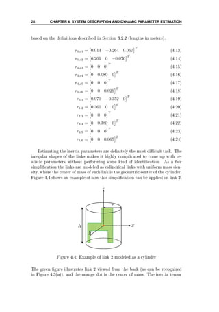
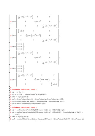
41. 4.4. PARAMETER ESTIMATION 29
of such a cylinder is shown in [4] to be
I =


1
12 mh2
+ 1
4 mr2
0 0
0 1
12 mh2
+ 1
4 mr2
0
0 0 1
2 mr2

 (4.25)
where m is the mass, r is the radius and h is the height of the cylinder. The cross
products are identically zero such that the inertia tensor becomes a diagonal
matrix in its principal axis form.
Determining the the mass, radius and height of the cylinders is kind of a
constrained task, where the constraints are that the total mass must be 98 kg
(including the base), and that the radius and height of the cylinders match
the dimensions of the manipulator given in Figure 4.3. Like the actual links
do, the cylinders will also overlap each other since the centers of mass are not
geometrically right in between two frames, and it was assumed uniform mass
density.
It is fair to believe that the mass density of every link is approximately equal.
The links are constructed of a shell of metal with components such as motors,
gearboxes, cables and belts on the inside. In addition, large proportions of
the total volume is just air in between these components. By a trial-and-error
approach, the masses, radii and heights was eventually found to match the
physical shape of the manipulator using a mutual mass density of 1500 kg
m3 . The
parameter values are given in Table 4.1, where the missing mass of 23 kg is
allocated the manipulator base. To make a comparison, the mass density of
steel is 7850 kg
m3 according to [12]. That is for massive steel, such that assuming
a mass density of the links of about the fth the mass density for steel seems
satisfying.
Link Mass Radius Height
1 27 kg 0.147 m 0.264 m
2 22 kg 0.108 m 0.402 m
3 - - -
4 25 kg 0.094 m 0.600 m
5 - - -
6 1 kg 0.054 m 0.072 m
Table 4.1: Cylinder parameters
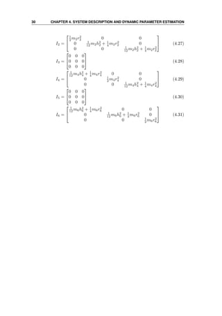
Note that the orientation of the attached frame determines the coordination
of the principal moments of inertia. With regard to this, the resulting inertia
tensors are calculated by substituting in (4.25). The result becomes
I1 =


1
12 m1h2
1 + 1
4 m1r2
1 0 0
0 1
2 m1r2
1 0
0 0 1
12 m1h2
1 + 1
4 m1r2
1

 (4.26)

42. 30 CHAPTER 4. SYSTEM DESCRIPTION AND DYNAMIC PARAMETER ESTIMATION
I2 =


1
2 m2r2
2 0 0
0 1
12 m2h2
2 + 1
4 m2r2
2 0
0 0 1
12 m2h2
2 + 1
4 m2r2
2

 (4.27)
I3 =


0 0 0
0 0 0
0 0 0

 (4.28)
I4 =


1
12 m4h2
4 + 1
4 m4r2
4 0 0
0 1
2 m4r2
4 0
0 0 1
12 m4h2
4 + 1
4 m4r2
4

 (4.29)
I5 =


0 0 0
0 0 0
0 0 0

 (4.30)
I6 =


1
12 m6h2
6 + 1
4 m6r2
6 0 0
0 1
12 m6h2
6 + 1
4 m6r2
6 0
0 0 1
2 m6r2
6

 (4.31)

43. Chapter 5
The Dynamic Model
The recursive Newton-Euler formulation was derived in general in Chapter 3.
Then in Chapter 4, a system description of the IRB 140 was presented. A sym-
bolic representation showed how to interpret the manipulator as a kinematic
chain, corresponding rotation matrices were calculated, and parameter estima-
tions were performed. To derive the dynamic model of the manipulator, the
rotation matrices and parameters from the system description are substituted
in the equations for the Newton-Euler formulation of an n-link manipulator.
The forward and backward recursions are carried out in Section 5.1 and 5.2
respectively, and comments on the results are found in Section 5.3.
With its six degrees of freedom, even the simplied system is quite complex.
Actually, the nal torque equations in the model are so huge that they do
not even suit to be shown in this text. Therefore, to let this chapter be clear
and easy to follow, all equations are kept in their recursive form. Appendix C
shows how the model has been computed in Maple by adjusting the framework
presented in Section 3.2.3 and Appendix B.
5.1 Forward Recursion
The forward recursion describes the linear and angular motion of of the links,
starting with link 1 and ending with link 6. The algorithm is described in
Section 3.2.2, and it is just a matter of substituting in the general equations for
an n-link manipulator.
As a part of the forward recursion it is necessary to compute bi, the axis
of rotation for each joint i expressed in frame i. Prior to the recursions, these
computations will be carried out right away for all joints to emphasize a great
advantage of the Newton-Euler formulation. The rotation axis in frame 0 is
given directly as
z0 = 0 0 1
T
(5.1)
31

44. 32 CHAPTER 5. THE DYNAMIC MODEL
and then the rotation axes for the joints are computed by Equation (3.30) as
b1 = (R0
1)T
z0 = 0 −1 0
T
(5.2)
b2 = (R0
2)T
R0
1z0 = 0 0 1
T
(5.3)
b3 = (R0
3)T
R0
2z0 = 0 −1 0
T
(5.4)
b4 = (R0
4)T
R0
3z0 = 0 1 0
T
(5.5)
b5 = (R0
5)T
R0
4z0 = 0 1 0
T
(5.6)
b6 = (R0
6)T
R0
5z0 = 0 0 1
T
(5.7)
Due to the coupled kinematics, these rotation axes will normally be functions of
q just like the rotation matrices. They will depend on how the coordinate frames
are dened, and therefore directly inuence the eciency of the Newton-Euler
formulation. By inspecting how the frames are dened in Figure 4.2, it can be
seen that when looking from frame i into frame i−1, the angular velocity ωi does
not depend on qi itself, but completely on the axis of rotation. Consequently
the rotation axes bi are not depending on q.
Link 1
The initial conditions are
ω0 = α0 = ac,0 = ae,0 = 0 (5.8)
Angular velocity and acceleration are calculated from Equation (3.29) and (3.33)
respectively, and becomes
ω1 = b1 ˙q1 (5.9)
α1 = b1 ¨q1 + ω1 × b1 ˙q1 (5.10)
Acceleration of the end of the link and the center of the link are calculated from
Equation (3.38) and (3.37) respectively, and becomes
ae,1 = ˙ω1 × r0,1 + ω1 × (ω1 × r0,1) (5.11)
ac,1 = ˙ω1 × r0,c1 + ω1 × (ω1 × r0,c1) (5.12)
Link 2
Substituting in the same equations as for link 1, the angular velocity and accel-
eration becomes
ω2 = (R1
2)T
ω1 + b2 ˙q2 (5.13)
α2 = (R1
2)T
α1 + b2 ¨q2 + ω2 × b2 ˙q2 (5.14)
Acceleration of the center and the end of the link becomes
ae,2 = (R1
2)T
ae,1 + ˙ω2 × r1,2 + ω2 × (ω2 × r1,2) (5.15)
ac,2 = (R1
2)T
ae,1 + ˙ω2 × r1,c2 + ω2 × (ω2 × r1,c2) (5.16)

45. 5.2. BACKWARD RECURSION 33
Link 3
Substituting for link 3 gives
ω3 = (R2
3)T
ω2 + b3 ˙q3 (5.17)
α3 = (R2
3)T
α2 + b3 ¨q3 + ω3 × b3 ˙q3 (5.18)
ae,3 = (R2
3)T
ae,2 (5.19)
ac,3 = (R2
3)T
ae,2 (5.20)
Link 4
Substituting for link 4 gives
ω4 = (R3
4)T
ω3 + b4 ˙q4 (5.21)
α4 = (R3
4)T
α3 + b4 ¨q4 + ω4 × b4 ˙q4 (5.22)
ae,4 = (R3
4)T
ae,3 + ˙ω4 × r3,4 + ω4 × (ω4 × r3,4) (5.23)
ac,4 = (R3
4)T
ae,3 + ˙ω4 × r3,c4 + ω4 × (ω4 × r3,c4) (5.24)
Link 5
Substituting for link 5 gives
ω5 = (R4
5)T
ω4 + b5 ˙q5 (5.25)
α5 = (R4
5)T
α4 + b5 ¨q5 + ω5 × b5 ˙q5 (5.26)
ae,5 = (R4
5)T
ae,4 (5.27)
ac,5 = (R4
5)T
ae,4 (5.28)
Link 6
Substituting for link 6 gives
ω6 = (R5
6)T
ω5 + b6 ˙q6 (5.29)
α6 = (R5
6)T
α5 + b6 ¨q6 + ω6 × b6 ˙q6 (5.30)
ac,6 = (R5
6)T
ae,5 + ˙ω6 × r5,c6 + ω6 × (ω6 × r5,c6) (5.31)
Note that there is no need to compute ae,6 because ae,i is only used to compute
ae,i+1 (and there is no link 7).
5.2 Backward Recursion
The backward recursion calculates the forces and joint torques acting on the
links, starting with link 6 and ending with link 1. Determining the joint torques
is the ultimate goal of the Newton-Euler formulation, because the torques are

46. 34 CHAPTER 5. THE DYNAMIC MODEL
the externally applied input to the model. As for the forward recursion, the
algorithm is described in Section 3.2.2 and it is just a matter of substituting in
the general equations for an n-link manipulator. Note that the force equation
includes the gravity vector. This gravity vector diers for each link, but can
easily be calculated with the use of rotation matrices as shown in the recursions
below.
Link 6
The terminal conditions are
f7 = τ7 = 0 (5.32)
The gravity vector becomes
g6 = (R0
6)T
g0 (5.33)
where g0 is the gravity vector in the inertial frame dened as
g0 = 0 0 −g
T
(5.34)
The force and joint torque exerted on the link are calculated from Equation
(3.24) and (3.27) respectively, and becomes
f6 = m6ac,6 − m6g6 (5.35)
τ6 = −f6 × r5,c6 + ω6 × (I6ω6) + I6α6 (5.36)
Link 5
Following the same procedure as for link 6, the gravity vector for link 5 becomes
g5 = (R0
5)T
g0 (5.37)
and the force and joint torque equations become
f5 = R5
6f6 (5.38)
τ5 = R5
6τ6 + ω5 × (I5ω5) + I5α5 (5.39)
Link 4
Substituting for link 4 gives
g4 = (R0
4)T
g0 (5.40)
f4 = R4
5f5 + m4ac,4 − m4g4 (5.41)
τ4 = R4
5τ5 − f4 × r3,c4 + R4
5f5 × r4,c4 + ω4 × (I4ω4) + I4α4 (5.42)

47. 5.3. COMMENTS 35
Link 3
Substituting for link 3 gives
g3 = (R0
3)T
g0 (5.43)
f3 = R3
4f4 (5.44)
τ3 = R3
4τ4 + ω3 × (I3ω3) + I3α3 (5.45)
Link 2
Substituting for link 2 gives
g2 = (R0
2)T
g0 (5.46)
f2 = R2
3f3 + m2ac,2 − m2g2 (5.47)
τ2 = R2
3τ3 − f2 × r1,c2 + R2
3f3 × r2,c2 + ω2 × (I2ω2) + I2α2 (5.48)
Link 1
Substituting for link 1 gives
g1 = (R0
1)T
g0 (5.49)
f1 = R1
2f2 + m1ac,1 − m1g1 (5.50)
τ1 = R1
2τ2 − f1 × r0,c1 + R1
2f2 × r1,c1 + ω1 × (I1ω1) + I1α1 (5.51)
5.3 Comments
The results in this chapter are interesting and veries why the Newton-Euler
formulation often is the preferred choice for manipulators with many degrees of
freedom. The recursive algorithm is easy to implement and consequently there
are small chances of doing any mistakes in the derivation. Strange behavior of
the model can mostly be connected to the preparations such as the set-up of
the kinematic chain and the frames, rotation matrices, vector denitions and
inertia tensors.
Note that even though link 3 and 5 have zero length and mass, they still have
to be considered in the recursions. The Newton-Euler formulation is based on
a kinematic chain with only single degree-of-freedom joints, such that n degrees
of freedom always lead to n steps in each recursion. However, some terms in
the expressions for link 3 and 5 are canceled out.
As mentioned in Section 3.1.1, the Newton-Euler formulation and the Euler-
Lagrange formulation can provide dierent insights. One interesting insight
in the Newton-Euler formulation comes from the nal joint torque vectors in
the backward recursion. All joints in the kinematic chain are single degree-of-
freedom joints, such that the torques applied are scalars about the rotation axes
computed in Equations (5.2)-(5.7). The other two elements of the torque vectors

48. 36 CHAPTER 5. THE DYNAMIC MODEL
can be explained as follows. When applying torque to any of the joints, this will
also generate torque components about the other axes of the joints due to the
coupled kinematics in the system. These torque components are not included
in the dynamic model because they do not induce motion (not aecting q),
but still it is valuable information about the physics of the manipulator. If the
joints in the manipulator are not constructed to physically resist these torque
quantities, the joints will break.
Although utilizing the Newton-Euler formulation appears to be quite easy,
the complexity of the resulting model should be emphasized. The basic idea be-
hind recursion is that the solution to a problem depends on solutions to smaller
instances on the same problem. The backward recursion of link 1 depends on
the backward recursion of link 2, which depends of the backwards recursion of
link 3, and so on. All in all the backward recursion of link 1 is directly depen-
dent on all 11 steps back to the forward recursion of link 1. Thus it should not
be a surprise that calculating τ1 from Equation (5.51) results in a huge vector.
To demonstrate the complexity of the system, the nal expression for τ1 (only
the component that induces motion) can be found in Appendix C. All details
are available to the reader by exploring the model that can be found in the
attached ZIP-le.

49. Chapter 6
Simulations and Results
This chapter deals with simulations of the dynamic model in open loop and
closed loop. Note that the goal is to perform simulations to prove the validity
of the model, not to optimize a control system for a specic job task.
The simulation structure in Simulink and the connection to Matlab is de-
scribed in Section 6.1. In Section 6.2 the second-order model is reduced to an
equivalent rst-order model which is needed to perform simulations in Simulink.
The open loop case is presented in Section 6.3 and 6.4. First the model is
driven with desired torque to check for open loop stability, and then energy
properties are investigated. The closed loop case in Section 6.5 presents a
mathematical proof of global asymptotic stability with PD control of a system
model in the form (3.1). Then the proof is veried for the model of the IRB
140.
6.1 Simulation Structure
In Simulink a so-called Level-2 Matlab S-Function is used to implement the
dynamics. This is a block with multiple input and output ports where input 1
is the state vector, input 2 is the applied torque vector, and the output is the
vector of state derivatives. For each time step in the simulation the updated
vector of state derivatives is computed from the new inputs. The contents of
the Level-2 Matlab S-Function block is the dynamic model in reduced form (see
Section 6.2). The Dormand-Prince method ode45 with relative tolerance 1−6
is
used for solving the dierential equations.
For each time step in the simulation, the state vector is sent from Simulink
to the Matlab interface through a To Workspace block. That makes it possible
to present the results graphically, and use the states to compute kinetic and
potential energy.
37

50. 38 CHAPTER 6. SIMULATIONS AND RESULTS
6.2 Reduced System Order
As described in Section 3.1, the dynamic model can be written on matrix form
as
M(q)¨q + C(q, ˙q) ˙q + g(q) = u (6.1)
To simulate the system in Simulink it is necessary to express it in the rst-order
nonlinear form
˙x = f(x, u) (6.2)
where x is the state vector and u is the torque vector.
The rst step is to rearrange the terms in (6.1) to get
¨q = M−1
(−C ˙q − g + u) (6.3)
where it is assumed that the inertia matrix M is invertible. The inertia matrix
is the main factor of the kinetic energy expression 1
2 ˙qT
M(q) ˙q (see Section 6.4.1).
Positive deniteness of M is seen directly by the fact that the kinetic energy is
always nonnegative, and is zero if and only if all the joint velocities are zero.
Thus, M is invertible and Equation (6.3) is valid.
The second step is to reduce the system from 6 second-order equations to
12 rst-order equations. Dening
x1 = q1, x2 = ˙x1 = ˙q1 (6.4)
x3 = q2, x4 = ˙x3 = ˙q2 (6.5)
...
...
x11 = q6, x12 = ˙x11 = ˙q6 (6.6)
the dynamic system can be expressed in the form (6.2) as
˙x1 = x2 (6.7)
˙x2 = f2(x, u) (6.8)
˙x3 = x4 (6.9)
˙x4 = f4(x, u) (6.10)
˙x5 = x6 (6.11)
˙x6 = f6(x, u) (6.12)
˙x7 = x8 (6.13)
˙x8 = f8(x, u) (6.14)
˙x9 = x10 (6.15)
˙x10 = f10(x, u) (6.16)
˙x11 = x12 (6.17)
˙x12 = f12(x, u) (6.18)
where f2i(x, u) is the expression for ¨qi in Equation (6.3) for i = 1, 2, ..., 6 and
substituting with x for q and ˙q.

51. 6.3. OPEN LOOP WITH DESIRED TORQUE 39
Note that this rst-order model is only how the dynamics are implemented
in Simulink and Matlab. All gures and text for the rest of this chapter will
refer to the original second-order system with q as the state vector.
6.3 Open Loop with Desired Torque
In open loop there is no feedback from the system output. In other words,
no information about the joint variables and its derivatives is available when
computing the input torque. Figure 6.1 shows the open loop model in Simulink,
where the block called irb140 contains all the dynamics.
Due to the excitation of gravity on the links being dependent on the joint
variables, it is quite intuitive that controlling the system in open loop is impos-
sible. The behavior of the system can be studied by driving the system with
the desired torque, that is the constant torque derived when substituting in the
dynamic equations for the desired joint variables and derivatives. If ˙qdes = 0,
this control torque can be explained as the constant torque which is needed to
keep the manipulator steady in the desired position.
To Workspace
states
States
Level−2 M−file
S−Function
irb140
Integrator
1
s
Input torque vector
0
Figure 6.1: Open loop simulink model
6.3.1 Simulations
The desired position and velocity are set to
qdes = 0 π
2 −π
2 0 0 0
T
(6.19)
˙qdes = 0 0 0 0 0 0
T
(6.20)
which is the position when the manipulator arm is stretched out to the maximum
in the x0-direction (see Figure 4.2). By substituting the desired position and
velocity in the dynamic equations ( ˙qdes gives ¨qdes = 0), the control torque

52. 40 CHAPTER 6. SIMULATIONS AND RESULTS
becomes
udes =








0
−2.409 · g − 13.782 · g
−2.409 · g
0
−0.029 · g
0








(6.21)
From an intuitive perspective this control torque is as expected. To keep the
manipulator steady in the chosen desired position, joint 2, 3 and 5 will have
to be actuated to compensate for the gravity, based on the law of action and
reaction. Joint 1, 4 and 6 will not be inuenced by gravity as long as ˙q = 0,
and is therefore given zero control torque.
Four simulations, each with dierent initial conditions, shows the behavior
of the system when applied this control torque. The gravity acceleration is set
to g = 9.81m
s2 , the gravity of earth.
Simulation 1
Initial conditions are set to
qinit = 0 0 0 0 0 0
T
(6.22)
˙qinit = 0 0 0 0 0 0
T
(6.23)
The response shown in Figure 6.2.
Simulation 2
Initial conditions are set to
qinit = 0 π −π
2 0 0 0
T
(6.24)
˙qinit = 0 0 0 0 0 0
T
(6.25)
The response is shown in Figure 6.3.
Simulation 3
Initial conditions are set to
qinit = 0 π
2 −π
2 0 0 0
T
(6.26)
˙qinit = 0 0 0 0 0 0
T
(6.27)
The response is shown in Figure 6.4.

53. 6.3. OPEN LOOP WITH DESIRED TORQUE 41
Simulation 4
Initial conditions are set to
qinit = 0 π
2 + 0.05 −π
2 0 0 0
T
(6.28)
˙qinit = 0 0 0 0 0 0
T
(6.29)
The response is shown in Figure 6.5.
6.3.2 Comments
Simulation 1 and 2 show a clearly unstable behavior when attempting to control
the system to a desired position that is not in immediate proximity to the initial
conditions. As mentioned, this is just as expected because the excitation of
gravity on the links is dependent on the joint variables.
In simulation 3, the initial conditions are equal to the desired position and ve-
locity, and the graph is showing the expected response. The joints are actuated
exactly as required to compensate for the gravity and to keep the manipulator
steady in the desired state. An interesting result is observed in simulation 4
where the initial position is only 0.05 radians (in joint 2) away from the desired
position. The rst four seconds looks exactly as in simulation 3, but suddenly
the system collapses into completely unstable behavior like in simulation 1 and
2.
The conclusion corresponds to what was assumed in advance of the simula-
tions. The behavior of the system is unstable, and just the slightest disturbance
in the system leads to a completely uncontrollable motion because the gravity
on the links is dependent on the joint variables, and the input is computed
without observing the output. The system requires feedback controllers to be
stabilized.

54. 42 CHAPTER 6. SIMULATIONS AND RESULTS
0 0.5 1 1.5 2 2.5 3 3.5 4 4.5 5
−20
−15
−10
−5
0
5
10
15
20
Time [s]
Radians
Response of q
q1
q
2
q3
q
4
q5
q
6
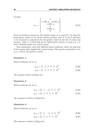
Figure 6.2: Open loop response with desired torque, simulation 1
0 0.5 1 1.5 2 2.5 3 3.5 4 4.5 5
−20
−15
−10
−5
0
5
10
15
20
Time [s]
Radians
Response of q
q
1
q2
q3
q
4
q5
q
6
Figure 6.3: Open loop response with desired torque, simulation 2

55. 6.3. OPEN LOOP WITH DESIRED TORQUE 43
0 1 2 3 4 5 6 7 8 9 10
−5
−4
−3
−2
−1
0
1
2
3
4
5
Time [s]
Radians
Response of q
q1
q
2
q3
q
4
q5
q
6
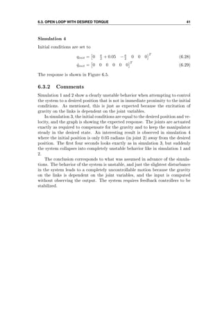
Figure 6.4: Open loop response with desired torque, simulation 3
0 1 2 3 4 5 6 7 8 9 10
−20
−15
−10
−5
0
5
10
15
20
Time [s]
Radians
Response of q
q
1
q2
q3
q
4
q5
q
6
Figure 6.5: Open loop response with desired torque, simulation 4

56. 44 CHAPTER 6. SIMULATIONS AND RESULTS
6.4 Energy Properties
The internal energy of the system is the sum of kinetic and potential energy.
It increases as energy is supplied and decreases as energy dissipates. The only
supplied energy in the model is the joint torque from the AC-motors, and no
dissipations are taken into account. As a result, the internal energy of the system
should be conserved during any motion as long as no torque is applied. Note
however that in a perfect model there would be dissipations from for instance
joint friction.
6.4.1 Kinetic Energy
The kinetic energy of a rigid object is the sum of two terms, the translational
kinetic energy obtained by concentrating the entire mass of the object at the
center of mass, and rotational kinetic energy of the body about the center of
mass. Mathematically, it is given as
K =
1
2
mvT
v +
1
2
ωT
Iω (6.30)
where m is the mass of the object, v and ω are the linear and angular velocity
vectors respectively, and I is the inertia tensor (see [20]).
For an n-link manipulator, the overall kinetic energy is the sum of the kinetic
energy for each link. It can be shown that the overall kinetic energy equals
K =
1
2
˙qT
M(q) ˙q (6.31)
where M is the conguration dependent inertia matrix recognized from the
general model in Equation (6.1). This is described in more detail in [20] on
page 250-254. Since the dynamic model is already derived in Chapter 5, it
is straightforward to compute the kinetic energy expression by substitution of
M in Equation (6.31). The resulting expression is huge and can be found in
Appendix C.
6.4.2 Potential Energy
The overall potential energy of an n-link manipulator is the sum of the potential
energy for each link. Given that the links are rigid, the only source of potential
energy is gravity. The overall potential energy can then be calculated as
P =
n
i=1
Pi =
n
i=1
mighci (6.32)
where n is the number of links, mi is the mass of link i, g is the gravitational
acceleration, and hci is the height of the center of mass of link i with respect to
a chosen zero level.

57. 6.4. ENERGY PROPERTIES 45
With the origin of frame 0 as the zero level, the potential energy is computed
as
P1 = m1 · g · −r0,c1,y (6.33)
P2 = m2 · g · [−r0,1,y + r1,c2,x · cos(q2)] (6.34)
P3 = 0 (6.35)
P4 = m4 · g · [−r0,1,y + r1,2,x · cos(q2) + r3,c4,y · sin(−q3 − q2)] (6.36)
P5 = 0 (6.37)
P6 = m6 · g · [−r0,1,y + r1,2,x · cos(q2) + r3,4,y · sin(−q3 − q2) (6.38)
+ r5,c6,z · sin(−q5 − q3 − q2)]
P = P1 + P2 + P4 + P6 (6.39)
where the third index added to the length vectors indicates the component of
the vector. Since link 3 and 5 have zero mass, their potential energy is zero as
well.
6.4.3 Pendulum Comparison
Simulating the system without any input makes an interesting comparison. The
system can now be interpreted as a complex 3D-pendulum with four joints and
four links, where two of the joints are ball joints (2 DOF) and the other two
joints are revolute joints (1 DOF). Multiple linked pendulums have received a
lot of attention from scientists because these systems are so easily constructed
yet the behavior is extremely complicated. Even the simplest multiple linked
pendulum, the double pendulum (2 DOF), is proved to be a chaotic system
[18] and [2]. A chaotic system is sensitive to initial conditions, meaning that
innitesimal changes to the initial conditions in an otherwise perfect experiment
will produce widely dierent results. It is not possible to predict the behavior,
and it is a complex question to determine when any of the links will ip (if
possible).
6.4.4 Simulations
It is fair to assume that the 3D-pendulum (6 DOF) will also be a chaotic sys-
tem, as it can be interpreted as a double pendulum with additional degrees of
freedom. Two simulations with very small changes in initial conditions show
the responses in the joint variables, as well as the energy in the system during
motion.

58. 46 CHAPTER 6. SIMULATIONS AND RESULTS
Simulation 1
Initial conditions and joint torques are set to
q = 0 0 0 0 0 0
T
(6.40)
˙q = 0 0 0 0 0 0
T
(6.41)
τ = 0 0 0 0 0 0
T
(6.42)
The response in joint variables are shown in Figure 6.6 and the energy is shown
in Figure 6.7.
Simulation 2
Initial conditions and joint torques are set to
q = 0 0.000001 0 0 0 0
T
(6.43)
˙q = 0 0 0 0 0 0
T
(6.44)
τ = 0 0 0 0 0 0
T
(6.45)
The response in joint variables are shown in Figure 6.8 and the energy is shown
in Figure 6.9.
6.4.5 Comments
These simulations conrm the expected chaotic behavior when the manipulator
is interpreted as a 3D-pendulum. The dierence in initial conditions is only
0.000001 radians (in joint 2), and the two simulations show entirely dierent
responses of the joint variables.
In addition, the energy plots provide some really valuable information. The
variations in kinetic and potential are dierent for the simulations, and is in
accordance to the motion of the manipulator. Still, the total energy is constant
in both simulations, and this conrms that the internal energy is conserved dur-
ing the motion as it should be with zero torque applied. However, by studying
the energy plots closely it can be observed that there are some small varia-
tions in the total energy. These variations are caused by numerical error when
Matlab solves the dierential equations, and would not be the case in a perfect
experiment.
This section has presented some outstanding observations, which close to
conrm that the derivation of the dynamic model is correct.

59. 6.4. ENERGY PROPERTIES 47
0 5 10 15 20 25 30
−100
−80
−60
−40
−20
0
20
40
60
80
100
Time [s]
Radians
Response of q
q1
q
2
q3
q
4
q5
q
6
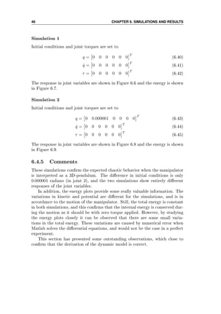
Figure 6.6: Open loop response with zero torque, simulation 1
0 5 10 15 20 25 30
0
50
100
150
200
250
300
350
400
450
Time[s]
Energy[J]
Internal energy
Kinetic energy
Potential energy
Total energy
Figure 6.7: Energy in the system with zero torque, simulation 1

60. 48 CHAPTER 6. SIMULATIONS AND RESULTS
0 5 10 15 20 25 30
−100
−80
−60
−40
−20
0
20
40
60
80
100
Time [s]
Radians
Response of q
q1
q
2
q3
q
4
q5
q
6
Figure 6.8: Open loop response with zero torque, simulation 2
0 5 10 15 20 25 30
0
50
100
150
200
250
300
350
400
450
Time[s]
Energy[J]
Internal energy
Kinetic energy
Potential energy
Total energy
Figure 6.9: Energy in the system with zero torque, simulation 2

61. 6.5. CLOSED LOOP POSITION CONTROL 49
6.5 Closed Loop Position Control
The open loop analysis with desired torque in Section 6.3 showed that control-
ling the system in open loop is impossible. This section deals with the attempt
of controlling the system in closed loop. In closed loop, feedback controllers
observe the output and calculate the error between this output and a reference.
To achieve desired output, controllers can take one or more of three standard
control elements that were described in Section 2.4.
Closed loop position control is also called the set-point tracking problem.
The goal is to demonstrate that the manipulator can move from the position
given as initial conditions, position A, to the position given as the reference
value, position B. The joint torque input is continuously calculated by the feed-
back controllers. The path taken from A to B, as well as how long the motion
lasts, is not controlled in the set-point tracking problem.
Section 6.5.1 presents a mathematical proof showing that a simple PD con-
trol structure works great for position control of systems in the general form
(6.1). Then in Section 6.5.2, PD controllers are added to the model in Simulink,
and simulations verify that the system is stable and that the position control is
satisfying.
6.5.1 Proof: PD control with gravity compensation
It is a remarkable fact that the simple PD scheme for set-point control can be
shown to work in the general case of a system model in the form of Equation
(6.1). This can be proved in a Lyapunov stability analysis, as shown in [20] and
[17]. This proof is of such importance and relevance to this thesis that it will
be restated in this section.
The proof is based on independent joint control, which means that each
joint is controlled as a single-input/single-output (SISO) system. Adding PD
controllers in the model, the input torque u can be written in vector form as
u = −Kp(qref − q) − Kd ˙q = −Kp ˜q − Kd ˙q (6.46)
where ˜q is the error between the joint references and the actual joint variables,
and Kp and Kd are positive denite diagonal matrices of proportional and
derivative gains.
It can be assumed that the gravitational acceleration is constant and known,
such that g(q) can be computed explicitly for all instants. By adding g(q) to the
input, gravity compensation is achieved such that the complete system model
is now given by
M(q)¨q + C(q, ˙q) ˙q + g(q) = u (6.47)
M(q)¨q + C(q, ˙q) ˙q + g(q) = −Kp ˜q − Kd ˙q + g(q) (6.48)
M(q)¨q + C(q, ˙q) ˙q = −Kp ˜q − Kd ˙q (6.49)

62. 50 CHAPTER 6. SIMULATIONS AND RESULTS
To show that the input torque given in Equation (6.48) achieves asymptotic
tracking, consider the Lyapunov function candidate
V =
1
2
˙qT
M(q) ˙q +
1
2
˜qT
Kp ˜q (6.50)
For the manipulator, V represents the total energy that would result if the
actuators were replaced by springs with stiness constants represented by Kp,
and with equilibrium position in qref . Thus, V is a positive function except in
the equilibrium position q = qref with ˙q = 0, at which point V is zero. If it can
be shown that V is decreasing along any motion, this implies that the robot is
moving toward that equilibrium position.
Noting that qref is constant, the derivative of V is given by
˙V = ˙qT
M(q)¨q +
1
2
˙qT ˙M(q) ˙q + ˙qT
Kp ˜q (6.51)
Solving for M(q)¨q in Equation (6.47) and substituting into the (6.51) yields
˙V = ˙qT
(u − C(q, ˙q) ˙q − g(q)) +
1
2
˙qT ˙M(q) ˙q + ˙qT
Kp ˜q (6.52)
= ˙qT
(u − g(q) + Kp ˜q) +
1
2
˙qT
[ ˙M(q) − 2C(q, ˙q)] ˙q (6.53)
= ˙qT
(u − g(q) + Kp ˜q) (6.54)
where ˙M(q) − 2C(q, ˙q) is skew symmetric1, and Equation (2.11) then gives
˙qT
[ ˙M(q) − 2C(q, ˙q)] ˙q = 0. Substituting the input torque in Equation (6.48) for
u in (6.54) above yields
˙V = − ˙qT
Kd ˙q ≤ 0 (6.55)
The above analysis shows that V is decreasing as long as ˙q is not zero.
Moreover it is necessary to prove that the manipulator can not reach a
position where ˙q = 0 but q = qref . Suppose ˙V ≡ 0, meaning that ˙V is zero
for all instants. Since Kd is positive denite, this implies that ˙q ≡ 0 and hence
¨q ≡ 0. Substituting this in the system model (6.49), the result becomes
0 = −Kp ˜q (6.56)
which implies that ˜q = 0. Finally, La Salle's theorem2then proves that the
equilibrium position q = qref is globally asymptotic stable.
It should be noted that if the gravitational terms g(q) are unknown, they
can not be added to the input because then the input cannot be computed.
Controlling the system would then require controllers with robust and adaptive
properties (see Section 6.5.3).
1The skew-symmetry of ˙M(q) − 2C(q, ˙q) is explained in [17], page 142-143
2La Salle's theorem is given in [20], page 456-457

63. 6.5. CLOSED LOOP POSITION CONTROL 51
6.5.2 Simulations with PD Control
The goal of this section is to perform simulations of the system with PD con-
trollers, checking for asymptotic stability. If this can be accomplished, the
mathematical proof in Section 6.5.1 is veried for the model. Figure 6.10 shows
the Simulink model of the system in closed loop. With gravity compensation
the model becomes
M(q)¨q + C(q, ˙q) ˙q = −Kp ˜q − Kd ˙q (6.57)
where the input is
u = −Kp ˜q − Kd ˙q (6.58)
Note that to increase the eciency of the simulations, it is chosen to remove
To Workspace2
tau To Workspace
states
Terminator2
Terminator1
States
Position reference vector
−C−
Level−2 M−file
S−Function
irb140
Kp
−K−
Kd
−K−
Integrator
1
s
Figure 6.10: Closed loop simulink model with PD controllers
the gravitational terms directly in the model (in the irb140 block) instead of
adding it to the input.
The mathematical proof gives no other bounds on Kp and Kd except for
being positive denite. Adjusting these controller gains optimally have not
been a priority, because it will not be decisive for global asymptotic stability.

64. 52 CHAPTER 6. SIMULATIONS AND RESULTS
A set of satisfying gain matrices was found as simple as
Kp =








50 0 0 0 0 0
0 50 0 0 0 0
0 0 50 0 0 0
0 0 0 50 0 0
0 0 0 0 50 0
0 0 0 0 0 60








(6.59)
Kd =








20 0 0 0 0 0
0 20 0 0 0 0
0 0 20 0 0 0
0 0 0 20 0 0
0 0 0 0 20 0
0 0 0 0 0 22








(6.60)
Three simulations with dierent initial conditions and reference values are pre-
sented to show the behavior of the system with these gains.
Simulation 1
Initial conditions and reference values are set to
qinit = 0 0 0 0 0 0
T
(6.61)
˙qinit = 0 0 0 0 0 0
T
(6.62)
qref = π
2 0 −π
2 π π
2 −π
T
(6.63)
The response in joint variables are shown in Figure 6.11 and the control input
is shown in Figure 6.12.
Simulation 2
Initial conditions and reference values are set to
qinit = 0 π −π
2 0 0 0
T
(6.64)
˙qinit = 0 0 0 0 0 0
T
(6.65)
qref = π 0 0 π −π
2 0
T
(6.66)
The response in joint variables are shown in Figure 6.13 and the control input
is shown in Figure 6.14.

65. 6.5. CLOSED LOOP POSITION CONTROL 53
Simulation 3
Initial conditions and reference values are set to
qinit = 0 π
2 −π
2 0 0 0
T
(6.67)
˙qinit = 0 0 0 0 0 0
T
(6.68)
qref = −π π −π −π −π
2 π
T
(6.69)
The response in joint variables are shown in Figure 6.15 and the control input
is shown in Figure 6.16.
6.5.3 Comments and Limitations
All simulations show that the states converge to the reference in about 3 seconds.
Asymptotic stability is veried, and the response is very satisfying. Neverthe-
less, several factors deserve to be emphasized. First of all, actuators cannot
supply innite torque. The nominal torque of the actuators and their gear ratio
limits the maximum input torque. This constraint can be included in Simulink
simply by saturating the input, but doing this is not necessary of reasons ex-
plained as follows. In the proof in Section 6.5.1 the gravitational terms g(q)
were added to the input because the gravitational acceleration was assumed to
be constant and known. With this simplication it is taken for granted that the
maximum input torque in the actuators is larger than g(q). The data sheets for
the IRB 140 do not state any torque values or other motor characteristics, but
obviously this assumption is valid since the manipulator is observed to beat
the gravity in a real environment. The mathematical proof gives no other
bounds on the input torque, thus global asymptotic stability is proved also for
saturated inputs. The only dierence in the simulations will be the increased
time to reach steady state.
Secondly, actuators cannot change the input torque value from τa to τb in
zero time. In other words, the input can never be a perfect step function.
The IRB 140 are controlled by electric AC-motors which supplies torque by
passing electricity to an electromagnet creating a magnetic eld. How fast this
magnetic eld is created will determine the maximum rate of change in input
torque. Rate limiters can be included in Simulink, but it is assumed that electric
motors create their electric elds very quickly. Consequently, rate limiters will
not make any signicant dierence in the simluations.
Some limitations have been chosen deliberately. First, joint friction is not
taken into account because of two reasons. First, it will be like a shot in the dark
to estimate the friction parameters without any given information. Secondly, it
does not really make a dierence to the simulations anyway when the input is not
saturated. However, if joint friction was to be taken into account, the simplest
way to include it would be to only model viscous friction, being proportional to
the joint velocity. The system model would then be
M(q)¨q + C(q, ˙q) + Fv ˙q + ˙q + g(q) = u (6.70)

66. 54 CHAPTER 6. SIMULATIONS AND RESULTS
where Fv is a diagnonal matrix of the joint friction coecients. This joint
friction material is taken from [1].
Note also that the simulations do not take into account the workspace of the
manipulator at all. Since the main goal of this chapter is to prove the validity
of the model, and not to optimize a control system for a specic job task, it
was found convenient to not include the workspace restrictions. The joints are
allowed to revolve freely, and no obstacles, oor, roof or walls are considered.
The data sheet (Appendix A) species the actual working range for the joints.
It should be mentioned that there exists several other control techniques and
methodologies that can be applied to the control of manipulators. The choice of
control structure should therefore match the requirements for the robot opera-
tion. If there are obstacles within the workspace of the manipulator, continuous
path tracking could be necessary to avoid collisions. Many operations may also
require that the manipulator moves from point A to point B in a precise xed
time interval. If the robot operation requires objects to be moved around, ro-
bust and adaptive controllers are superior. Note that this can often be the case
for the IRB 140, as it is designed to handle payloads of up to 6 kg. The me-
chanical design, motor characteristics, and problems due to backlash, friction
and gear reduction, may also aect the choice of control structure.

67. 6.5. CLOSED LOOP POSITION CONTROL 55
0 0.5 1 1.5 2 2.5 3 3.5 4 4.5 5
−4
−3
−2
−1
0
1
2
3
4
Time [s]
Radians
Response of q
q1
q
2
q3
q
4
q5
q
6
Figure 6.11: Closed loop position control response, simulation 1
0 0.5 1 1.5 2 2.5 3
−50
−40
−30
−20
−10
0
10
20
30
40
50
Time [s]
Torque[Nm]
Input torque
τ
1
τ2
τ
3
τ
4
τ5
τ6
Figure 6.12: Closed loop position control input, simulation 1

68. 56 CHAPTER 6. SIMULATIONS AND RESULTS
0 0.5 1 1.5 2 2.5 3 3.5 4 4.5 5
−2
−1
0
1
2
3
4
Time [s]
Radians
Response of q
q1
q
2
q3
q
4
q5
q
6
Figure 6.13: Closed loop position control response, simulation 2
0 0.5 1 1.5 2 2.5 3
−100
−80
−60
−40
−20
0
20
40
60
80
100
Time [s]
Torque[Nm]
Input torque
τ
1
τ2
τ
3
τ
4
τ5
τ6
Figure 6.14: Closed loop position control input, simulation 2

69. 6.5. CLOSED LOOP POSITION CONTROL 57
0 0.5 1 1.5 2 2.5 3 3.5 4 4.5 5
−4
−3
−2
−1
0
1
2
3
4
Time [s]
Radians
Response of q
q1
q
2
q3
q
4
q5
q
6
Figure 6.15: Closed loop position control response, simulation 3
0 0.5 1 1.5 2 2.5 3
−100
−80
−60
−40
−20
0
20
40
60
80
100
Time [s]
Torque[Nm]
Input torque
τ
1
τ2
τ
3
τ
4
τ5
τ6
Figure 6.16: Closed loop position control input, simulation 3

71. Chapter 7
Comparing the Results to the
Euler-Lagrange Model
The two main approaches for dynamic modeling of robot manipulators are the
Newton-Euler formulation and the Euler-Lagrange formulation. In Chapter
3.1.1 it was stated that there is no clear answer to the question of which of the
methods is better than the other, because of all the factors that inuence the
computation time. However, [7] proves at least that a recursive procedure is
more ecient than treating the manipulator as a whole.
The purpose of this chapter is to compare the behavior and computation
times of the model derived by the Newton-Euler formulation in this thesis,
to a model of the IRB 140 derived by the Euler-Lagrange formulation [13].
The latter was derived by the standard Euler-Lagrange procedure, meaning
the manipulator was treated as whole and analyzed based on its kinetic and
potential energy.
7.1 Remarks on the Direction of State Variables
The ideal situation for the comparison would be that all denitions of the kine-
matic chain as well as the parameters of system are equal in the two models.
This was originally the intention, and the frames and parameters in the Newton-
Euler model were dened deliberately to accomplish this. Unfortunately, it was
discovered by experimental simulations later on that the direction of change
in at least one state variable is dened opposite in the Euler-Lagrange model.
Referring to the representation of the Newton-Euler system in Figure 4.2, this
nding applies to q3, meaning the direction of positive q3 in the Euler-Lagrange
model is counter-clockwise when looking at that gure. Dening the subscript
ne for Newton-Euler and el for Euler-Lagrange, the following simulations con-
rm this discovery.
59

72. 60 CHAPTER 7. COMPARING THE RESULTS TO THE EULER-LAGRANGE MODEL
Simulation 1
The initial conditions and applied torque for the simulations in Figure 7.1 are
qne,init = 0 π −π
2 0 0 0
T
(7.1)
˙qne,init = 0 0 0 0 0 0
T
(7.2)
τne = 0 0 0 0 0 0
T
(7.3)
qel,init = 0 π π
2 0 0 0
T
(7.4)
˙qel,init = 0 0 0 0 0 0
T
(7.5)
τel = 0 0 0 0 0 0
T
(7.6)
As observed in the gures, the behavior of the two models are identical when
q3 has opposite signs. The initial conditions corresponds to the conguration
where the manipulator is hanging like a pendulum in a stable equilibrium point.
0 1 2 3 4 5 6 7 8 9 10
−1
0
1
2
3
4
Time [s]
Radians
Response of q in Euler−Lagrange
q
1
q
2
q
3
q
4
q5
q6
0 1 2 3 4 5 6 7 8 9 10
−2
−1
0
1
2
3
4
Time [s]
Radians
Response of q in Newton−Euler
q
1
q
2
q
3
q
4
q5
q6
Figure 7.1: Conrming opposite q3-direction, simulation 1

73. 7.1. REMARKS ON THE DIRECTION OF STATE VARIABLES 61
Simulation 2
The initial conditions and applied torque for the simulations in Figure 7.2 are
qne,init = 0 π π
2 0 0 0
T
(7.7)
˙qne,init = 0 0 0 0 0 0
T
(7.8)
τne = 0 0 0 0 0 0
T
(7.9)
qel,init = 0 π −π
2 0 0 0
T
(7.10)
˙qel,init = 0 0 0 0 0 0
T
(7.11)
τel = 0 0 0 0 0 0
T
(7.12)
The behavior of the models are now similar but not identical when q3 has op-
posite signs. The initial conditions corresponds to the conguration where link
2 is hanging straight down, while link 4 and 6 represents a double inverted pen-
dulum on top of link 2. As observed, the combination of gravity and numerical
error in the solver will eventually move the manipulator out of the unstable
equilibrium point. The dierence in state responses is simply caused by chaotic
behavior (see Section 6.4.3).
0 1 2 3 4 5 6 7 8 9 10
−20
−10
0
10
20
Time [s]
Radians
Response of q in Euler−Lagrange
q
1
q
2
q
3
q
4
q5
q6
0 1 2 3 4 5 6 7 8 9 10
−20
−10
0
10
20
Time [s]
Radians
Response of q in Newton−Euler
q
1
q
2
q
3
q
4
q5
q6
Figure 7.2: Conrming opposite q3-direction, simulation 2

74. 62 CHAPTER 7. COMPARING THE RESULTS TO THE EULER-LAGRANGE MODEL
7.2 Computation Times
The results in Section 7.1 conrm the dierence in direction of q3, but the
coupled kinematics make it hard to draw any conclusions about the direction
of other states in the Euler-Lagrange model. However, the variations in com-
putation time caused by dierent directions of state variables will not be of
any signicance. This section will investigate the eciency of the formulations
described in terms of computation times in open loop and closed loop. To dis-
tinguish clearly, the simulation time chosen in Simulink will be referred to as
simulation time, and the actual time recorded during the simulation will be
referred to as real time.
7.2.1 Open Loop
The simulations showed in Figure 7.2 are used to compare computation times
in open loop. The simulation time for both models were set to 10 seconds. The
real times were recorded as 7 minutes for the Euler-Lagrange model and only 6
seconds for the Newton-Euler model.
7.2.2 Closed loop
Three dierent simulations for the Newton-Euler model were performed in
closed loop with PD controllers (see Section 6.5.2). All of them showed that the
states converged to the reference in about 3 seconds of simulation time. The
total simulation times were 5 seconds for all simulations, and the real times
were recorded to be 28 minutes, 32 minutes and 27 minutes respectively.
Equivalent simulations in closed loop with PD controllers have been per-
formed with the Euler-Lagrange model, and the results are quite remarkable.
The simulations were awfully time-consuming and they required so much com-
puter capacity that it was chosen to stop the simulations after 2.3 seconds of
simulation time. The real time was then at about 18 hours for all three simu-
lations.
The three simulations for the Euler-Lagrange model are presented below.
Note that the transient responses diers from the the ones in the Newton-Euler
model because of the dierence in direction of state variables. Unfortunately,
2.3 seconds was just a little short simulation time to reach steady state, but
still the plots show enough to prove the same asymptotic stable behavior as for
the Newton-Euler model.
Simulation 1
Initial conditions and reference values are set equal to (6.61)-(6.63), and the
response is shown in Figure 7.3.

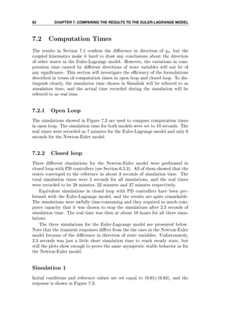
75. 7.2. COMPUTATION TIMES 63
Simulation 2
Initial conditions and reference values are set equal to (6.64)-(6.66), and the
response is shown in Figure 7.4.
Simulation 3
Initial conditions and reference values are set equal to (6.67)-(6.69), and the
response is shown in Figure 7.5.
7.2.3 Comments
All simulation times and recorded real times in this comparison are summarized
in Table 7.1. Several times throughout this thesis it has been pointed out that
a recursive procedure is faster than treating the manipulator as a whole. This
experiment underlines that statement to the full extent.
Simulation plot
Newton-Euler Euler-Lagrange
Sim. time Real time Sim. time Real time
Figure 7.2 10 s 6 s 10 s 7 m
Figure 6.11 and 7.3 5 s 28 m 2.3 s 18 h
Figure 6.13 and 7.4 5 s 32 m 2.3 s 18 h
Figure 6.15 and 7.5 5 s 27 m 2.3 s 18 h
Table 7.1: Computation times
0 0.5 1 1.5 2
−4
−3
−2
−1
0
1
2
3
4
Time [s]
Radians
q
q
1
q
2
q
3
q
4
q
5
q
6
Figure 7.3: Euler-Lagrange closed loop position control response, simulation 1

76. 64 CHAPTER 7. COMPARING THE RESULTS TO THE EULER-LAGRANGE MODEL
0 0.5 1 1.5 2
−2
−1
0
1
2
3
4
Time [s]
Radians
q
q
1
q
2
q3
q
4
q
5
q6
Figure 7.4: Euler-Lagrange closed loop position control response, simulation 2
0 0.5 1 1.5 2
−4
−3
−2
−1
0
1
2
3
4
Time [s]
Radians
q
q
1
q
2
q
3
q
4
q
5
q
6
Figure 7.5: Euler-Lagrange closed loop position control response, simulation 3

77. Chapter 8
Concluding Remarks
This chapter presents a concluding summary of the thesis, as well as recommen-
dations for improvement and usage of the results.
8.1 Conclusion
The topic of this thesis has been dynamic modeling and simulation of robot
manipulators. Dierent methods for dynamic modeling have been introduced,
with particular focus on the Newton-Euler formulation. The eciency and
advantages of the formulation have been compared to the characteristics of the
Euler-Lagrange formulation, although there could not be drawn a conclusion
to the question of which method is better than the other in general. The
computation time depends on several aspects in the system to be analyzed, and
the approaches provide dierent insights such that personal preference becomes
a factor as well.
It has been shown that estimating the dynamic parameters accurately is a
hard and time-consuming challenge. It requires either the possibility to measure
the state variables and its derivatives during motion of the manipulator, or
specic knowledge about other identication techniques as for example CAD
modeling. Even if such an attempt is to be performed, the dynamic parameters
will not be perfectly accurate. In the model for the IRB 140, the dynamic
parameters have been estimated based on inspecting the manipulator carefully,
making intuitive guesses when required.
Simulations of the dynamic model had as main purpose to prove the valid-
ity of the model. Open loop simulations with desired torque showed that the
behavior of the system was unstable just as assumed; the slightest disturbance
in the system led to a completely uncontrollable motion. Energy investigations
of the system with zero torque applied showed that the internal energy of the
system is constant during any motion as long as no dissipations of energy are
taken into account. That is an outstanding observation that really underlines
that the model is behaving correctly.
65

78. 66 CHAPTER 8. CONCLUDING REMARKS
Global asymptotic stability of the system with PD control and gravity com-
pensation was proved mathematically in a Lyapunov stability analysis. After-
wards, this was conrmed to be the case for the model by simulations with PD
control.
It was mentioned that the computation times of the Newton-Euler formu-
lation and Euler-Lagrange formulation depends on several factors. However, in
any case, it is a fact that a recursive procedure is more ecient than treating the
manipulator as a whole. By comparing simulations of the Newton-Euler model
and the Euler-Lagrange model of the IRB 140, this statement was proved to
hold in all cases.
8.2 Recommendations for Future Work
Derivation of dynamic models will in almost any case involve challenging pa-
rameter estimation. The dynamic parameters in this thesis are estimated quite
roughly, and accordingly there is much potential for improvement. Being able to
measure the state variables and its derivatives in experiments with the IRB 140
would be a huge step towards estimating the centers of mass and inertia tensors
quite accurately. If the torques can also be measured, for example by measuring
the current, it is actually possible to compute the parameters explicitly by the
identication method explained in Section 3.1.2.
The model in this thesis is also limited in other aspects. A perfect model
would contain dynamic eects like joint friction and joint exibility, and there
would be bounds on the maximum input torque for the motors. Actually, the
data sheet (see Appendix A) states the maximum velocity for each joint, such
that the maximum input torques can be calculated explicitly if motor speci-
cations are known.
Controller design should also be recommended for future work. Inverse dy-
namics control can be utilized for trajectory tracking of the manipulator. As
mentioned in Chapter 6, trajectory tracking could be required to avoid colli-
sions with obstacles within the workspace of the manipulator. Obviously the
workspace of the manipulator is bounded by the working range of the joints
(given in Appendix A) as well as the oor, the roof, and the walls, in addition
to possible obstacles. The main drawback with inverse dynamics is that the
dynamic parameters must be known, if not, the ideal performance is no longer
guaranteed. Robust and adaptive motion control is one way of overcoming this
problem. The goal of this kind of control is to maintain desired performance
despite parametric uncertainty. Thus, robust and adaptive control is superior
for robot operation that requires objects to be moved around by the robot arm.
If actions and improvements like mentioned above are performed, the model
attained might be good enough to achieve pretty accurate motion control of the
IRB 140. Being able to design a control system that can compete with ABB's
QuickMove and TrueMove systems would be the ultimate achievement. Unfor-
tunately, implementing the model cannot be accomplished as long as access to
the state variables and the controller in the manipulator is not granted.

79. Appendix A
IRB 140 Data Sheet
67

80. 68 APPENDIX A. IRB 140 DATA SHEET

81. IRB 140
Industrial Robot
Robotics
Main Applications
Arc welding
Assembly
Cleaning/Spraying
Machine tending
Material handling
Packing
Deburring
Small, Powerful and Fast
Compact, powerful IRB 140 industrial robot.
Six axis multipurpose robot that handles payload of 6 kg,
with long reach (810 mm). The IRB 140 can be floor mounted,
inverted or on the wall in any angle. Available as Standard,
FoundryPlus, Clean Room and Wash versions, all mechani-
cal arms completely IP67 protected, making IRB 140 easy to
integrate in and suitable for a variety of applications. Uniquely
extended radius of working area due to bend-back mecha-
nism of upper arm, axis 1 rotation of 360 degrees even as
wall mounted.
The compact, robust design with integrated cabling adds to
overall flexibility. The Collision Detection option with full path
retraction makes robot reliable and safe.
Using IRB 140T, cycle-times are considerably reduced where
axis 1 and 2 predominantly are used.
Reductions between 15-20 % are possible using pure axis
1 and 2 movements. This faster versions is well suited for
packing applications and guided operations together with
PickMaster.
IRB Foundry Plus and Wash versions are suitable for operat-
ing in extreme foundry environments and other harch environ-
ments with high requirements on corrosion resistance and
tightness. In addition to the IP67 protection, excellent surface
treatment makes the robot high pressure steam washable.
The white-finish Clean Room version meets Clean Room class
10 regulations, making it especially suited for environments
with stringent cleanliness standards.

82. ©CopyrightABBRobotics.PR10031EN_R8February2009.
www.abb.com/robotics
IRB 140
Specification
Robot versions Handling Reach of Remarks
capacity 5th axis
IRB 140/IRB 140T 6 kg 810 mm
IRB 140F/IRB 140TF 6 kg 810 mm Foundry Plus Protection
IRB 140CR/
IRB 140TCR 6 kg 810 mm Clean Room
IRB 140W/
IRB 140TW 6 kg 810 mm Wash Protection
Supplementary load (on upper arm alt. wrist)
on upper arm 1 kg
on wrist 0.5 kg
Number of axes
Robot manipulator 6
External devices 6
Integrated signal supply 12 signals on upper arm
Integrated air supply Max. 8 bar on upper arm
Performance
Position repeatability 0.03 mm (average result from ISO test)
Axis movement Axis Working range
1, C Rotation 360°
2, B Arm 200°
3, A Arm 280°
4, D Wrist Unlimited (400° default)
5, E Bend 240°
6, P Turn Unlimited (800° default)
Max. TCP velocity 2.5 m/s
Max. TCP acceleration 20 m/s2
Acceleration time 0-1 m/s 0.15 sec
Velocity
Axis no. IRB 140 IRB 140T
1 200°/s 250°/s
2 200°/s 250°/s
3 260°/s 260°/s
4 360°/s 360°/s
5 360°/s 360°/s
6 450°/s 450°/s
Cycle time
5 kg Picking side IRB 140 IRB 140T
cycle 25 x 300 x 25 mm 0,85s 0,77s
Electrical Connections
Supply voltage 200–600 V, 50/60 Hz
Rated power
Transformer rating 4.5 kVA
Power consumption typicly 0,4 kW
Physical
Robot mounting Any angle
Dimensions
Robot base 400 x 450 mm
Robot controller H x W x D 950 x 800 x 620 mm
Weight
Robot manipulator 98 kg
Environment
Ambient temperature for
Robot manipulator 5 – 45°C
Relative humidity Max. 95%
Degree of protection,
Manipulator IP67
Options Foundry
Wash (High pressure steam washable)
Clean Room, class 6
(certified by IPA)
Noise level Max. 70 dB (A)
Safety Double circuits with supervision,
emergency stops and safety
functions,
3-position enable device
Emission EMC/EMI-shielded
Data and dimensions may be changed without notice
Working range
810
65
670
70
380
1092
712
352
151
486
670
810
70
70
486
352
712
1092
380
65
670 810
70 486
352
1092
0
50
100
150
200
250
300
350
0 50 100 150 200 250
Z-distance(mm)
0
50
100
150
200
250
300
0 50 100 150 200 250 300
Z-distance(mm)
L-distance (mm)
L-distance (mm)
1,5 kg
2 kg
3 kg
4 kg
5 kg
6 kg
6,5 kg
6 kg
5 kg
4 kg
3 kg
0
50
100
150
200
250
300
350
0 50 100 150 200 250
Z-distance(mm)
0
50
100
150
200
250
300
0 50
Z-distance(mm)
L-distance (mm)
1,5 kg
2 kg
3 kg
4 kg
5 kg
6 kg
6,5 kg

83. Appendix B
Automated Framework
71

84. 72 APPENDIX B. AUTOMATED FRAMEWORK

85. Automated framework for deriving the dynamic model of robot
manipulators by the Newton-Euler formulation
This is an automated framework for deriving the dynamic model of robot manipulators by the Newton-
Euler formulation. The framework is restricted to manipulators with rigid links and only revolute joints,
but it can be adjusted to suit other kinds of manipulators if desired. The composition presented is for
three degrees of freedom, but due to the recursive procedure it can easily be adjusted to any number of
degrees of freedom.
Complex manipulators with several degrees of freedom will result in huge dynamic systems, and it
might be desirable to evaluate smaller parts of a system individually. Every element of the inertia
matrix, as well as the gravity components and the Coriolis and centrifugal components, are evaluated
individually towards the end of the framework. It is optional to define symbolic values if the goal is a
less specific model, but note that the more symbolic values and the less defined zeros, the larger
dynamic model.
The Matlab conversion code used in the end can be applied to any expression, and is a simple way to
convert Maple code to Matlab code. Note that the joint variable derivatives are not known in the Matlab
conversion code. These quantities will have to be redefined as desired in Matlab.
All quantities must be defined according to the standard convention of how a manipulator is interpreted.
In addition, it is important to add or remove lines following the recursive procedure, according to the
how many degrees of freedom there are in the manipulator to be analyzed. Explanations for the parts
that has to be adjusted (grayed out) are given below as well as in the code (green text).
Joint variables: Specify the number of joint variables (degrees of freedom) in the manipulator by
adjusting the q-vector.
Link length vectors and vectors to the centers of mass: Define the link length vectors and the vectors
to the centers of mass, which all are independent of configuration.
Gravity vector in inertial frame: Define the direction of gravity in the inertial frame (frame 0).
Rotation matrices: Define the rotation matrices describing rotations from every frame to the
subsequent frame.
Inertia matrices: Define the inertia tensors for the links. If the mass distribution of a link is symmetric
with respect to the attached frame, then the inertia tensor will be diagonal.
#Joint variables (degrees of freedom)
#TO DO: Specify the number of joint variables (degrees of freedom) in the
manipulator by adjusting the q-vector.
#Link length vectors and vectors to the centers of mass
#TO DO: Define the link length vectors and the vectors to the centers of
mass, which all are independent of configuration.

86. #Gravity vector in inertial frame
#TO DO: Define the direction of gravity in the inertial frame (frame 0).
#Rotation matrices
#TO DO: Define the rotation matrices describing rotations from every frame to
the subsequent frame.
#Inertia matrices
#TO DO: Define the inertia tensors for the links. If the mass distribution of
a link is symmetric with respect to the attached frame, then the inertia
tensor will be diagonal.
#Axis of rotation of joint i expressed in frame i

87. #Forward recursion: Link 1
#Forward recursion: Link 2
#Forward recursion: Link 3
#Backward recursion: Link 3
#Backward recursion: Link 2
#Backward recursion: Link 1

88. #The final dynamic system
#Evaluating smaller parts of the system
#Matlab conversion

89. Appendix C
IRB 140 Dynamic Model
77

90. 78 APPENDIX C. IRB 140 DYNAMIC MODEL

91. Dynamic Model of the IRB 140
#Defining joint variables
#Defining link length vectors
#Gravity vector in inertial frame
#Rotation matrices

92. #Axis of rotation of joint i expressed in frame i
#Link Masses
#Sylinder link dimensions
#Inertia matrices

93. #Forward recursion: Link 1
#Forward recursion: Link 2

94. #Forward recursion: Link 3
#Forward recursion: Link 4
#Forward recursion: Link 5
#Forward recursion: Link 6
#Backward recursion: Link 6

95. (1)(1)
#Backward recursion: Link 5
#Backward recursion: Link 4
#Backward recursion: Link 3
#Backward recursion: Link 2
#Backward recursion: Link 1

108. #Setting up the matrix elements

110. (2)(2)
#Setting up the dynamic system
#Kinetic energy

111. (2)(2)

114. #Matlab conversion

117. Appendix D
Errata in Chapter 7.6 in [20]
Chapter 7.6 Newton-Euler Formulation in [20] has some misleading notations
and errata. These are the ndings, and the suggested corrections.
• Page 275, denition of Ri
i+1 should be:
Ri
i+1 : the rotation matrix from frame i to frame i + 1.
• Page 276, denition of Ii should be:
Ii : the inertia tensor of link i about a frame parallel to frame i whose
origin is at the center of mass of link i.
• Page 276, denition of ri,ci should be:
ri−1,ci : the vector from the origin of frame i − 1 to the center of mass of
link i.
• Page 276, denition of ri+1,ci should be:
ri,ci : the vector from the origin of frame i to the center of mass of link i.
• Page 276, denition of ri,i+1 should be:
ri−1,i : the vector from the origin of frame i − 1 to the origin of frame i.
• Page 277, Equation (7.145) should be:
τi −Ri
i+1τi+1 +fi ×ri−1,ci −(Ri
i+1fi+1)×ri,ci = Iiαi +ωi ×(Iiωi) (D.1)
• Page 277, Equation (7.147) should be:
τi = Ri
i+1τi+1 −fi ×ri−1,ci +(Ri
i+1fi+1)×ri,ci +Iiαi +ωi ×(Iiωi) (D.2)
• Page 278, Equation (7.153) should be:
αi = (Ri−1
i )T
αi−1 + bi ¨qi + ωi × bi ˙qi (D.3)
105

118. 106 APPENDIX D. ERRATA IN CHAPTER 7.6 IN [20]
• Page 278, Equation (7.154) should be:
v
(0)
c,i = v
(0)
e,i−1 + ω
(0)
i × r
(0)
i−1,ci (D.4)
• Page 278, the sentence between (7.154) and (7.155) should be:
To obtain an expression for the acceleration, we note that the vector r
(0)
i−1,ci
is constant in frame i.
• Page 278, Equation (7.155) should be:
a
(0)
c,i = a
(0)
e,i−1 × r
(0)
i−1,ci + ω
(0)
i × (ω
(0)
i × r
(0)
i−1,ci) (D.5)
• Page 279, Equation (7.158) should be:
ac,i = (Ri−1
i )T
ae,i−1 + ˙ωi × ri−1,ci + ωi × (ωi × ri−1,ci) (D.6)
• Page 279, the sentence between Equation (7.158) and Equation (7.159)
should be:
Now, to nd the acceleration of the end of link i, we can use Equation
(7.158) with ri−1,i replacing ri−1,ci.
• Page 279, Equation (7.159) should be:
ae,i = (Ri−1
i )T
ae,i−1 + ˙ωi × ri−1,i + ωi × (ωi × ri−1,i) (D.7)
• Page 279, Equation (7.162) for ω2 should be:
ω2 = ( ˙q1 + ˙q2)k (D.8)
• Page 280, Equation (7.163) should be:
r0,c1 = lc1i, r1,c1 = (lc1 − l1)i, r0,1 = l1i (D.9)
• Page 280, Equation (7.164) should be:
r1,c2 = lc2i, r2,c2 = (lc2 − l2)i, r1,2 = l2i (D.10)
• Page 280, Equation (7.166) should be:
g1 = (R0
1)T
gj = −g


sin(q1)
cos(q1)
0

 (D.11)
• Page 280, Equation (7.168) should be:
ac,2 = (R1
2)T
ae,1 +(¨q1 + ¨q2)k ×lc2i+( ˙q1 + ˙q2)k ×[( ˙q1 + ˙q2)k ×lc2i] (D.12)

119. 107
• Page 281, Equation (7.169) should be:
(R1
2)T
ae,1 =
cos(q2) sin(q2)
−sin(q2) cos(q2)
−l1 ˙q2
1
l1 ¨q1
(D.13)
=
−l1 ˙q2
1cos(q2) + l1 ¨q1sin(q2)
l1 ˙q2
1sin(q2) + l1 ¨q1cos(q2)
(D.14)
• Page 281, Equation (7.170) should be:
ac,2 =
−l1 ˙q2
1cos(q2) + l1 ¨q1sin(q2) − lc2( ˙q1 + ˙q2)2
l1 ˙q2
1sin(q2) + l1 ¨q1cos(q2) + lc2(¨q1 + ¨q2)
(D.15)
• Page 281, Equation (7.171) should be:
g2 = −g
sin(q1 + q2)
cos(q1 + q2)
(D.16)
• Page 281, Equation (7.174) should be:
τ2 = I2(¨q1 + ¨q2)k + [m2l1lc2sin(q2) ˙q2
1 + m2l1lc2cos(q2)¨q1
+ m2l2
c2(¨q1 + ¨q2) + m2lc2gcos(q1 + q2)]k
(D.17)
• Page 282, Equation (7.175) should be:
f1 = R1
2f2 + m1ac,1 − m1g1 (D.18)
• Page 282, Equation (7.176) should be:
τ1 = R1
2τ2 − f1 × lc1i + (R1
2f2) × (lc1 − l1)i + I1α1 + ω1 × (I1ω1) (D.19)
• Page 282, second sentence after Equation (7.176) should be:
First, R1
2τ2 = τ2, since the rotation matrix does not aect the third com-
ponents of vectors.
• Page 282, Equation (7.177) should be:
τ1 = τ2 − m1ac,1 × lc1i + m1g1 × lc1i − (R1
2f2) × l1i + I1α1 (D.20)

121. Appendix E
Contents of Attached ZIP-File
PDF Files
• Master's Thesis: A digital copy of this thesis.
• Project Work 2010: A digital copy of [6].
• IRB 140 Data Sheet: A digital copy of [15].
• IRB 140 Product Specication: A digital copy of [16].
Maple Files
• 3dofFramework.mw: The automated framework.
• 6dofIRB140.mw: Derivation of the dynamic model of the IRB 140.
Matlab and Simulink Files
• SixDofOpenLoop.mdl: The open loop Simulink model.
• SixDofPDreg.mdl: The closed loop Simulink model with PD controllers.
• irb140.m: Matlab code of the dynamic model (the irb140 block).
• plot6dof.m: Matlab code creating the plots after a simulation.
109

123. Bibliography
[1] T. Bajd, M. Mihelj, J. Lenar£i£, A. Stanovnik, and M. Munih. Robotics.
Springer Verlag, 2010.
[2] G.L. Baker and J.A. Blackburn. The pendulum: a case study in physics.
Oxford University Press, USA, 2005.
[3] J.G. Balchen, T. Andresen, and B.A. Foss. Reguleringsteknikk. Institutt
for teknisk kybernetikk, 2004.
[4] M.F. Beatty. Principles of engineering mechanics. Springer Verlag, 2006.
[5] B. Dasgupta and P. Choudhury. A general strategy based on the Newton-
Euler approach for the dynamic formulation of parallel manipulators. Mech-
anism and Machine Theory, 34(6):801824, 1999.
[6] H. Høifødt. Dynamics of robot manipulators by the Newton-Euler formu-
lation, 5th year project work, 2010.
[7] J.M. Hollerbach. A Recursive Lagrangian Formulation of Maniputator
Dynamics and a Comparative Study of Dynamics Formulation Complexity.
Systems, Man and Cybernetics, IEEE Transactions on, 10(11):730736,
2007.
[8] H.K. Khalil. Nonlinear Systems 3rd. Prentice Hall, 2002.
[9] Maplesoft. Maple 15 - The Essential Tools for Mathematics and Modeling,
Last accessed June 13, 2011.
http://www.maplesoft.com/products/maple/index.aspx.
[10] Mathworks. MATLAB - The Language Of Technical Computing, Last ac-
cessed June 13, 2011.
http://www.mathworks.com/products/matlab/.
[11] Mathworks. Simulink - Simulation and Model-Based Design, Last accessed
June 13, 2011.
http://www.mathworks.com/products/simulink/.
[12] SI metric. Density of metals, Last accessed May 25, 2011.
http://www.simetric.co.uk/si_metals.htm.
111

124. 112 BIBLIOGRAPHY
[13] S. Pchelkin. Dynamic model of the irb 140 by the euler-lagrange formula-
tion.
[14] ABB Robotics. ABB Product Guide for IRB 140, Last accessed June 14,
2011.
http://www.abb.com/product/seitp327/7c4717912301eb02c1256efc00278a26.
aspx?productLanguage=nocountry=00.
[15] ABB Robotics. Data sheet for IRB 140, Retrieved September 21, 2010.
[16] ABB Robotics. Product specication for IRB 140, Retrieved September
21, 2010.
[17] L. Sciavicco and B. Siciliano. Modelling and control of robot manipulators.
Springer Verlag, 2000.
[18] T. Shinbrot, C. Grebogi, J. Wisdom, and J.A. Yorke. Chaos in a double
pendulum. American Journal of Physics, 60:491, 1992.
[19] W.M. Silver. On the equivalence of Lagrangian and Newton-Euler dy-
namics for manipulators. The International Journal of Robotics Research,
1(2):60, 1982.
[20] M.W. Spong, S. Hutchinson, and M. Vidyasagar. Robot modeling and
control. Wiley New Jersey, 2006.
[21] Adobe Systems. Adobe Illustrator, Last accessed June 13, 2011.
http://www.adobe.com/products/illustrator.html.
[22] J.R. Taylor. Classical mechanics. Univ Science Books, 2005.