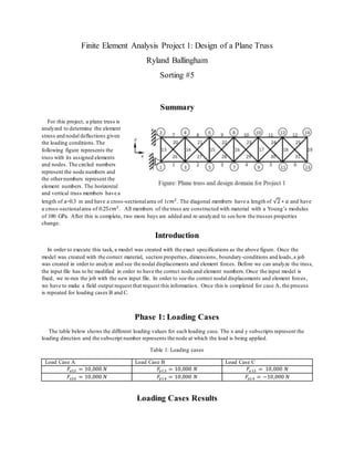
SlideShare a Scribd company logo
1 of 13
Finite Element Analysis Project 1: Design of a Plane Truss
Ryland Ballingham
Sorting #5
Summary
For this project, a plane truss is
analyzed to determine the element
stress and nodal deflections given
the loading conditions.The
following figure represents the
truss with its assigned elements
and nodes. The circled numbers
represent the node numbers and
the othernumbers represent the
element numbers. The horizontal
and vertical truss members have a
length of a=0.3 m and have a cross-sectionalarea of 1𝑐𝑚2
. The diagonal members have a length of √2 ∗ 𝑎 and have
a cross-sectionalarea of 0.25𝑐𝑚2
. All members of the truss are constructed with material with a Young’s modulus
of 100 GPa. After this is complete, two more bays are added and re-analyzed to see how the trusses properties
change.
Introduction
In order to execute this task, a model was created with the exact specifications as the above figure. Once the
model was created with the correct material, section properties, dimensions, boundary-conditions and loads,a job
was created in order to analyze and see the nodal displacements and element forces. Before we can analyze the truss,
the input file has to be modified in order to have the correct node and element numbers. Once the input model is
fixed, we re-run the job with the new input file. In order to see the correct nodal displacements and element forces,
we have to make a field output request that request this information. Once this is completed for case A, the process
is repeated for loading cases B and C.
Phase 1: Loading Cases
The table below shows the different loading values for each loading case. The x and y subscripts represent the
loading direction and the subscript number represents the node at which the load is being applied.
Table 1: Loading cases
Load Case A Load Case B Load Case C
𝐹𝑥13 = 10,000 𝑁 𝐹𝑦13 = 10,000 𝑁 𝐹𝑥13 = 10,000 𝑁
𝐹𝑥14 = 10,000 𝑁 𝐹𝑦14 = 10,000 𝑁 𝐹𝑥14 = −10,000 𝑁
Loading Cases Results
Table 2: Elements Stresses/Forces for each loading case
The force values were calculated knowing that the cross-sectionalarea of elements 1-19 is 1 𝑐𝑚2
and elements 20-
31 is 0.25 𝑐𝑚2
. These values were multiplied using excel by the stress values obtained in Abaqus to get the force
values.
Table 3: Load Case A displacements
Node number Magnitude U (m) U1 displacement (m) U2 displacement (m)
1 2.17472E-05 1E-32 2.17472E-05
2 0 1E-32 0
3 0.000280111 0.000278253 3.22118E-05
4 0.00027845 0.000278253 -1.04646E-05
Element
number
Element
Stress
(Case A)
(Pa)
Element
Stress
(Case B)
(Pa)
Element
Stress
(Case C)
(Pa)
Element
Force
(Case C)
(N)
Element
Force
(Case B)
(N)
Element
Force
(Case C)
(N)
1 9.28E+07 1.10E+09 1.00E+08 9275.09 110376 10000
2 9.30E+07 9.00E+08 1.00E+08 9302.36 89985.9 10000
3 9.30E+07 7.00E+08 1.00E+08 9301.33 70000.5 10000
4 9.30E+07 5.00E+08 1.00E+08 9301.33 50000 10000
5 9.30E+07 3.00E+08 1.00E+08 9302.36 30000 10000
6 9.28E+07 1.00E+08 1.00E+08 9275.09 10000 10000
7 9.28E+07 -1.10E+09 -1.00E+08 9275.09 -109624 -10000
8 9.30E+07 -9.00E+08 -1.00E+08 9302.36 -90014.1 -10000
9 9.30E+07 -7.00E+08 -1.00E+08 9301.33 -69999.5 -10000
10 9.30E+07 -5.00E+08 -1.00E+08 9301.33 -50000 -10000
11 9.30E+07 -3.00E+08 -1.00E+08 9302.36 -30000 -10000
12 9.28E+07 -1.00E+08 -1.00E+08 9275.09 -10000 -10000
13 -7.25E+06 -9.62E+07 2.26E-08 -724.905 -9623.92 2.25875E-12
14 -1.42E+07 3.62E+06 0.00E+00 -1422.55 361.94 0
15 -1.40E+07 -1.36E+05 0.00E+00 -1396.31 -13.612 0
16 -1.40E+07 5.12E+03 -1.73E-07 -1397.33 0.511925 -1.73472E-11
17 -1.40E+07 -1.93E+02 3.47E-07 -1396.31 -0.0192527 3.46945E-11
18 -1.42E+07 7.24E+00 -3.47E-07 -1422.55 0.000724101 -3.46945E-11
19 -7.25E+06 -2.83E-01 0.00E+00 -724.905 -2.82552E-05 0
20 4.10E+07 5.44E+08 -1.41E-07 1025.17 13610.275 -3.52365E-12
21 3.95E+07 5.66E+08 -4.34E-08 986.615 14162.15 -1.0842E-12
22 3.95E+07 5.66E+08 8.67E-08 988.065 14141.375 2.16841E-12
23 3.95E+07 5.66E+08 0.00E+00 988.065 14142.175 0
24 3.95E+07 5.66E+08 -5.20E-07 986.615 14142.125 -1.30104E-11
25 4.10E+07 5.66E+08 -2.08E-06 1025.17 14142.125 -5.20418E-11
26 4.10E+07 -5.87E+08 9.76E-08 1025.17 -14674 2.43946E-12
27 3.95E+07 -5.65E+08 -2.17E-08 986.615 -14122.125 -5.421E-13
28 3.95E+07 -5.66E+08 -8.67E-08 988.065 -14142.9 -2.16841E-12
29 3.95E+07 -5.66E+08 8.67E-08 988.065 -14142.1 2.16841E-12
30 3.95E+07 -5.66E+08 6.94E-07 986.615 -14142.125 1.73472E-11
31 4.10E+07 -5.66E+08 2.08E-06 1025.17 -14142.125 5.20418E-11
5 0.000558231 0.000557324 3.18182E-05
6 0.000557415 0.000557324 -1.00711E-05
7 0.000836969 0.000836364 3.18336E-05
8 0.000836424 0.000836364 -1.00864E-05
9 0.00111586 0.0011154 3.18182E-05
10 0.00111545 0.0011154 -1.00711E-05
11 0.00139485 0.00139447 3.22118E-05
12 0.00139451 0.00139447 -1.04646E-05
13 0.00167287 0.00167273 2.17472E-05
14 0.00167273 0.00167273 -5.24483E-18
Table 4: Load Case B displacements
Node number Magnitude U (m) U1 displacement (m) U2 displacement (m)
1 0.000288717 1.2E-31 0.000288717
2 0 -1.2E-31 2E-32
3 0.00759309 0.00331128 0.00683304
4 0.00759307 -0.00328872 0.0068439
5 0.0204367 0.00601086 0.0195328
6 0.02043 -0.00598914 0.0195324
7 0.0379046 0.00811087 0.0370267
8 0.0379 -0.00808913 0.0370267
9 0.0589101 0.00961087 0.0581208
10 0.0589065 -0.00958913 0.0581208
11 0.082289 0.0105109 0.0816149
12 0.0822862 -0.0104891 0.0816149
13 0.106857 0.0108109 0.106309
14 0.106855 -0.0107891 0.106309
Table 4: Load Case C displacements
Node number Magnitude U (m) U1 displacement (m) U2 displacement (m)
1 0 1E-32 -6.77626E-20
2 0 -1E-32 0
3 0.000424264 0.0003 0.0003
4 0.000424264 -0.0003 0.0003
5 0.00134164 0.0006 0.0012
6 0.00134164 -0.0006 0.0012
7 0.00284605 0.0009 0.0027
8 0.00284605 -0.0009 0.0027
9 0.00494773 0.0012 0.0048
10 0.00494773 -0.0012 0.0048
11 0.00764853 0.0015 0.0075
12 0.00764853 -0.0015 0.0075
13 0.010949 0.0018 0.0108
14 0.010949 -0.0018 0.0108
Fig. 1. Deformed displacement plot of load case A.
Fig. 2. Deformed Stress plot of load case A.
Fig. 3. Deformed displacement plot of load case B.
Fig. 4. Deformed stress plot of load case B.
Fig. 5. Deformed displacement plot of load case C.
Fig. 6. Deformed stress plot of load case C (note bottomof truss is in tension and the top portion is in compression)
Phase 2: Equivalent Properties for 6-bay
If we assume that the truss behaves likes a cantilever beam, cross-sectionalproperties of the truss can be found.
The three properties that we are concerned with include: Axial rigidity (𝐸𝐴 𝑒𝑞 ), flexural rigidity (𝐸𝐼 𝑒𝑞) and shear
rigidity (𝐺𝐴 𝑒𝑞 ). The meaning of these properties can be found in the following table.
Table 5: Equivalent Properties
Axial rigidity (𝐸𝐴 𝑒𝑞 ) A measure of a materials ability to oppose and resist
deformation due to axial forces.
Flexural rigidity (𝐸𝐼 𝑒𝑞) A measure of a materials ability to oppose and resist
deformation due to bending.
Shear rigidity (𝐺𝐴 𝑒𝑞 ) A measure of a materials ability to oppose and resist
deformation due to shearforces.
Equivalent Property Results
Load Case A
Using the first loading case, the axial rigidity can be solved due to the axial loading conditions using the following
formula:
𝐸𝐴 𝑒𝑞 =
𝐹𝐿
𝑢 𝑡𝑖𝑝
(1)
Since we know F = 20,000 N (sum of the two forces), L = 1.8 m and the average tip deflection (𝑢 𝑡𝑖𝑝 ) from abaqus =
0.001673 m. Plugging these numbers (1) yields a value of 𝐸𝐴 𝑒𝑞 = 21,518 kN.
Load Case C
Using loading case C, we can solve for the flexural rigidity due to the applied couple at the end of the beam using
the following formula:
𝐸𝐼 𝑒𝑞 =
𝐶𝐿2
2𝑣𝑡𝑖𝑝
(2)
To solve for the applied couple (C), we use the following formula:
𝐶 = 𝐹 × 𝑑
Where F = 10,000 N and d (distance between the applied forces (F)) = 0.3 m. Plugging these numbers in yields a
couple of C=3,000 N-m. The length (L) is the same as loading case A (1.8 m) and the average tip deflection (𝑣𝑡𝑖𝑝 )
from abaqus = 0.010949 m. Plugging these values into (2) yields a value of 𝐸𝐼 𝑒𝑞 = 443,879 N or about 444 kN.
Load Case B
Since we solved for flexural rigidity in load case C, we can solve for the shearrigidity (𝐺𝐴 𝑒𝑞 ) due to the transverse
F using the following formula:
𝐺𝐴 𝑒𝑞 =
𝐹𝐿
𝑣𝑡𝑖𝑝 −
𝐹𝐿3
3𝐸𝐼 𝑒𝑞
(3)
Since F = 20,000 N, L = 1.8 m, 𝐸𝐼 𝑒𝑞 = 443,879 N and 𝑣𝑡𝑖𝑝 from abaqus = 0.106856 m we can solve for the shear
rigidity. Plugging these values into (3) yields a value of 𝐺𝐴 𝑒𝑞 = 1,869,300 Pa. or 1.9 MPa
Phase 3: Extended Bay
In this portion of the project, the beam model was verified by adding two more bays. This was accomplished by
modifying the input file by adding more nodes and more elements in the same manner as the 6-bay design. For this
new model, load cases A-C were applied just as before (except the forces were applied at the new, extended tip).
The following table shows the results that were obtained for the displacements. Note: The new nodes follow the
same pattern as the original models nodes.
Extended Bay Results
Table 6: Load Case A displacements (extended bay)
Node number Magnitude U (m) U1 displacement (m) U2 displacement (m)
1 2.17472E-05 1E-32 2.17472E-05
2 0 1E-32 0
3 0.000280111 0.000278253 3.22118E-05
4 0.00027845 0.000278253 -1.04646E-05
5 0.000558231 0.000557324 3.18182E-05
6 0.000557415 0.000557324 -1.00711E-05
7 0.000836969 0.000836364 3.18336E-05
8 0.000836424 0.000836364 -1.00864E-05
9 0.00111586 0.0011154 3.18182E-05
10 0.00111545 0.0011154 -1.00711E-05
11 0.00139485 0.00139447 3.22121E-05
12 0.00139451 0.00139447 -1.04649E-05
13 0.00167287 0.00167273 2.17398E-05
14 0.00167273 0.00167273 7.40093E-09
15 0.00195128 0.00195101 3.25909E-05
16 0.00195104 0.00195101 -1.08437E-05
17 0.0022294 0.00222929 2.17324E-05
18 0.00222929 0.00222929 1.4791E-08
Table 7: Load Case B displacements (extended bay)
Node number Magnitude U (m) U1 displacement (m) U2 displacement (m)
1 0.000288717 1.6E-31 0.000288717
2 0 -1.6E-31 2E-32
3 0.00921311 0.00451128 0.00803304
4 0.00921156 -0.00448872 0.0080439
5 0.0257454 0.00841086 0.0243328
6 0.025738 -0.00838914 0.0243324
7 0.0492396 0.0117109 0.0478267
8 0.0492344 -0.0116891 0.0478267
9 0.0786523 0.0144109 0.0773208
10 0.0786483 -0.0143891 0.0773208
11 0.11283 0.0165109 0.111615
12 0.112826 -0.0164891 0.111615
13 0.15059 0.0180109 0.149509
14 0.150587 -0.0179891 0.149509
15 0.190743 0.0189109 0.189803
16 0.190741 -0.0188891 0.189803
17 0.232094 0.0192109 0.231297
18 0.232092 0.00222929 1.4791E-08
Table 8: Load Case C displacements (extended bay)
Node number Magnitude U (m) U1 displacement (m) U2 displacement (m)
1 4.91279E-19 1E-32 4.91279E-19
2 0 -1E-32 0
3 0.000424264 0.0003 0.0003
4 0.000424264 -0.0003 0.0003
5 0.00134164 0.0006 0.0012
6 0.00134164 -0.0006 0.0012
7 0.00284605 0.0009 0.0027
8 0.00284605 -0.0009 0.0027
9 0.00494773 0.0012 0.0048
10 0.00494773 -0.0012 0.0048
11 0.00764853 0.0015 0.0075
12 0.00764853 -0.0015 0.0075
13 0.010949 0.0018 0.0108
14 0.010949 -0.0018 0.0108
15 0.0148492 0.0021 0.0147
16 0.0148492 -0.0021 0.0147
17 0.0193494 0.0024 0.0192
18 0.0193494 -0.0024 0.0192
Fig. 6. Extended bay deformed displacements of load case A
Fig. 7. Extended bay deformed displacements of load case B
Fig. 8. Extended bay deformed displacements of load case C
FEA model and equivalent property comparison
Table 9: 6-bay equivalent properties
Property 6-bay model
Axial rigidity (𝐸𝐴 𝑒𝑞 ) 21,518 kN
Flexural rigidity (𝐸𝐼 𝑒𝑞) 443,879 N
Shear rigidity (𝐺𝐴 𝑒𝑞 ) 1.869 MPa
Table 10: End node displacement comparison
Load Case FEA model method Equivalent Property calculation
Load Case A 0.002229 m 0.002231 m
Load Case B 0.232093 m 0.233302 m
Load Case C 0.0192 m 0.019493 m
The equivalent properties were calculated the same way as in phase 2 of this report. For the 8-bay design,the length
was increased to 2.4 m from 1.8 m and the tip deflections were different as well (these tip deflections were the
average deflections at nodes 17 and 18 instead of at nodes 13 and 14). Table 10 shows that whether doing the
calculations for the tip deflections by hand or by using the FEA model, the results are similar.
Load Case B (6-bay) Fully-Stressed Design Results
Given that the allowable stress is 600 MPa and that we know the old stress/area values for load case B, a new
minimum cross-sectionalarea can be calculated using the following formula (4):
𝐴 𝑛𝑒𝑤
𝑒
=
𝜎 𝑜𝑙𝑑
𝑒
𝜎 𝑎𝑙𝑙𝑜𝑤𝑎𝑏𝑙𝑒
𝑒 𝐴 𝑜𝑙𝑑
𝑒
(4)
Table 10: Load Case B fully stressed design
Element number Old Stress (𝜎 𝑜𝑙𝑑)
(MPa)
Old Area (𝐴 𝑜𝑙𝑑 )( 𝑚2
) New Stress
(𝜎 𝑛𝑒𝑤) (MPa)
New Area
(𝐴 𝑛𝑒𝑤 )( 𝑐𝑚2
)
1 1103.76 0.0001 602.974 1.8396
2 899.859 0.0001 596.796 1.499765
3 700.005 0.0001 601.607 1.166675
4 500 0.0001 598.716 0.833333333
5 300 0.0001 601.174 0.5
6 100 0.0001 598.507 0.166666667
7 -1096.24 0.0001 -597.005 1.827066667
8 -900.141 0.0001 -603.203 1.500235
9 -699.995 0.0001 -418.893 1.166658333
10 -500 0.0001 -601.308 0.833333333
11 -300 0.0001 -598.826 0.5
12 -100 0.0001 -601.493 0.166666667
13 -96.2392 0.0001 -565.894 0.160398667
14 3.6194 0.0001 428.446 0.006032333 (0.01)
15 -0.13612 0.0001 -306.708 0.000226867 (0.01)
16 0.00511925 0.0001 79.0079 8.53208E-06 (0.01)
17 -0.000192527 0.0001 -50.2687 3.20878E-07 (0.01)
18 7.24101E-06 0.0001 33.8309 1.20684E-08 (0.01)
19 -2.82552E-07 0.0001 -24.8756 4.7092E-10 (0.01)
20 544.411 0.000025 565.894 0.226837917
21 566.486 0.000025 628.792 0.236035833
22 565.655 0.000025 588.753 0.235689583
23 565.687 0.000025 606.537 0.235702917
24 565.685 0.000025 596.478 0.235702083
25 565.685 0.000025 601.493 0.235702083
26 -586.96 0.000025 -631.633 0.244566667
27 -564.885 0.000025 -571.127 0.23536875
28 -565.716 0.000025 -611.246 0.235715
29 -565.684 0.000025 -593.463 0.235701667
30 -565.685 0.000025 602.974 0.235702083
31 -565.685 0.000025 596.796 0.235702083
Above shows the new stress values (from abaqus)and the new minimum cross-sectionalareas to achieve a fully
stressed design.Element numbers 14, 15, 16,17,18,19 would have to have a minimum cross-sectionalarea of 0.01
𝑐𝑚2
(since any area smaller than 0.01 𝑐𝑚2
cannot be achieved due to manufacturing reasons).
Fig. 9. Deformed fully-stressed load case B
Fig. 10. Deformed displacements of fully-stressed load case B
Discussion
It appears that increasing the length of a beam (while keeping everything else constant)increases axial rigidity
and flexural rigidity and decreases shearrigidity. This needs to be taken into consideration when designing
beams/trusses in order to prevent potential failure.
Anotherphenomena that I noticed is that when the bay size is increased, the magnitude of the average nodal
displacements increases as well for all loading cases.
In addition, whether using equivalent properties method or a FEM model, the values for the displacements are
similar. This shows that Abaqus does a great job at conveying correct data when performing analysis.
References
[1] EML 4507 Project 1.pdf
[2] Beer, Ferdinand P., and E. Russell Johnston. Mechanics of Materials.New York: McGraw-Hill, 1981. Print.

More Related Content

What's hot

Tellegen’s-Substitution-Reciprocity-Theorem.ppt
Tellegen’s-Substitution-Reciprocity-Theorem.pptTellegen’s-Substitution-Reciprocity-Theorem.ppt
Tellegen’s-Substitution-Reciprocity-Theorem.pptHussain K
 
Lab 8 tensile testing
Lab 8 tensile testing  Lab 8 tensile testing
Lab 8 tensile testing elsa mesfin
 
STRENGTH OF MATERIALS for beginners
STRENGTH OF MATERIALS for  beginnersSTRENGTH OF MATERIALS for  beginners
STRENGTH OF MATERIALS for beginnersmusadoto
 
Ch 04 MATLAB Applications in Chemical Engineering_陳奇中教授教學投影片
Ch 04 MATLAB Applications in Chemical Engineering_陳奇中教授教學投影片Ch 04 MATLAB Applications in Chemical Engineering_陳奇中教授教學投影片
Ch 04 MATLAB Applications in Chemical Engineering_陳奇中教授教學投影片Chyi-Tsong Chen
 
C4 Lab Report 5 Fluid Mechanics.pdf
C4 Lab Report 5 Fluid Mechanics.pdfC4 Lab Report 5 Fluid Mechanics.pdf
C4 Lab Report 5 Fluid Mechanics.pdfMUHAMMADSYAHMIMAWARD
 
fundamentals of electrical engineering
 fundamentals of electrical engineering fundamentals of electrical engineering
fundamentals of electrical engineeringayushi kesarvani
 
Elements constitutifs du_plan_de_protection_hta
Elements constitutifs du_plan_de_protection_htaElements constitutifs du_plan_de_protection_hta
Elements constitutifs du_plan_de_protection_htaimene imene
 
Attachments 2012 03_13
Attachments 2012 03_13Attachments 2012 03_13
Attachments 2012 03_13arslan_akbar90
 
Basics of Integration and Derivatives
Basics of Integration and DerivativesBasics of Integration and Derivatives
Basics of Integration and DerivativesFaisal Waqar
 
Electrotechnique : Exercices corrigés
Electrotechnique : Exercices corrigésElectrotechnique : Exercices corrigés
Electrotechnique : Exercices corrigésRAMZI EL IDRISSI
 
6161103 3.4 three dimensional force systems
6161103 3.4 three dimensional force systems6161103 3.4 three dimensional force systems
6161103 3.4 three dimensional force systemsetcenterrbru
 
Harmonically+excited+vibration
Harmonically+excited+vibrationHarmonically+excited+vibration
Harmonically+excited+vibrationRodrigo Tucunduva
 
Castigliano’s Method
Castigliano’s MethodCastigliano’s Method
Castigliano’s Methodaapx
 
Vector differentiation, the ∇ operator,
Vector differentiation, the ∇ operator,Vector differentiation, the ∇ operator,
Vector differentiation, the ∇ operator,Tarun Gehlot
 
Solution manual for introduction to finite element analysis and design nam ...
Solution manual for introduction to finite element analysis and design   nam ...Solution manual for introduction to finite element analysis and design   nam ...
Solution manual for introduction to finite element analysis and design nam ...Salehkhanovic
 

What's hot (20)

H#8
H#8H#8
H#8
 
Tellegen’s-Substitution-Reciprocity-Theorem.ppt
Tellegen’s-Substitution-Reciprocity-Theorem.pptTellegen’s-Substitution-Reciprocity-Theorem.ppt
Tellegen’s-Substitution-Reciprocity-Theorem.ppt
 
Lab 8 tensile testing
Lab 8 tensile testing  Lab 8 tensile testing
Lab 8 tensile testing
 
STRENGTH OF MATERIALS for beginners
STRENGTH OF MATERIALS for  beginnersSTRENGTH OF MATERIALS for  beginners
STRENGTH OF MATERIALS for beginners
 
Examen RDM 2014-2015
Examen RDM 2014-2015Examen RDM 2014-2015
Examen RDM 2014-2015
 
Finite Difference Method
Finite Difference MethodFinite Difference Method
Finite Difference Method
 
Ch 04 MATLAB Applications in Chemical Engineering_陳奇中教授教學投影片
Ch 04 MATLAB Applications in Chemical Engineering_陳奇中教授教學投影片Ch 04 MATLAB Applications in Chemical Engineering_陳奇中教授教學投影片
Ch 04 MATLAB Applications in Chemical Engineering_陳奇中教授教學投影片
 
C4 Lab Report 5 Fluid Mechanics.pdf
C4 Lab Report 5 Fluid Mechanics.pdfC4 Lab Report 5 Fluid Mechanics.pdf
C4 Lab Report 5 Fluid Mechanics.pdf
 
fundamentals of electrical engineering
 fundamentals of electrical engineering fundamentals of electrical engineering
fundamentals of electrical engineering
 
Elements constitutifs du_plan_de_protection_hta
Elements constitutifs du_plan_de_protection_htaElements constitutifs du_plan_de_protection_hta
Elements constitutifs du_plan_de_protection_hta
 
Attachments 2012 03_13
Attachments 2012 03_13Attachments 2012 03_13
Attachments 2012 03_13
 
Basics of Integration and Derivatives
Basics of Integration and DerivativesBasics of Integration and Derivatives
Basics of Integration and Derivatives
 
Electrotechnique : Exercices corrigés
Electrotechnique : Exercices corrigésElectrotechnique : Exercices corrigés
Electrotechnique : Exercices corrigés
 
6161103 3.4 three dimensional force systems
6161103 3.4 three dimensional force systems6161103 3.4 three dimensional force systems
6161103 3.4 three dimensional force systems
 
Harmonically+excited+vibration
Harmonically+excited+vibrationHarmonically+excited+vibration
Harmonically+excited+vibration
 
Castigliano’s Method
Castigliano’s MethodCastigliano’s Method
Castigliano’s Method
 
torsion
torsiontorsion
torsion
 
Vector differentiation, the ∇ operator,
Vector differentiation, the ∇ operator,Vector differentiation, the ∇ operator,
Vector differentiation, the ∇ operator,
 
Som strain energy
Som strain energySom strain energy
Som strain energy
 
Solution manual for introduction to finite element analysis and design nam ...
Solution manual for introduction to finite element analysis and design   nam ...Solution manual for introduction to finite element analysis and design   nam ...
Solution manual for introduction to finite element analysis and design nam ...
 

Similar to FEA_project1

EGME 306A The Beam Page 1 of 18 Group 2 EXPER.docx
EGME 306A  The Beam Page 1 of 18 Group 2 EXPER.docxEGME 306A  The Beam Page 1 of 18 Group 2 EXPER.docx
EGME 306A The Beam Page 1 of 18 Group 2 EXPER.docxSALU18
 
Advanced mathematical analysis of chassis integrated platform designed for un...
Advanced mathematical analysis of chassis integrated platform designed for un...Advanced mathematical analysis of chassis integrated platform designed for un...
Advanced mathematical analysis of chassis integrated platform designed for un...Dr.Vikas Deulgaonkar
 
Sriram1000991882-Report-FractureMechanics
Sriram1000991882-Report-FractureMechanicsSriram1000991882-Report-FractureMechanics
Sriram1000991882-Report-FractureMechanicsSriram Sambasivam
 
ME 5720 Fall 2015 - Wind Turbine Project_FINAL
ME 5720 Fall 2015 - Wind Turbine Project_FINALME 5720 Fall 2015 - Wind Turbine Project_FINAL
ME 5720 Fall 2015 - Wind Turbine Project_FINALOmar Latifi
 
IRJET- Non-Linear Contact Analysis and Design Optimisation of Load Cell for H...
IRJET- Non-Linear Contact Analysis and Design Optimisation of Load Cell for H...IRJET- Non-Linear Contact Analysis and Design Optimisation of Load Cell for H...
IRJET- Non-Linear Contact Analysis and Design Optimisation of Load Cell for H...IRJET Journal
 
Twice yield method for assessment of fatigue life assesment of pressure swing...
Twice yield method for assessment of fatigue life assesment of pressure swing...Twice yield method for assessment of fatigue life assesment of pressure swing...
Twice yield method for assessment of fatigue life assesment of pressure swing...Kingston Rivington
 
Examples on stress distribution
Examples on stress distributionExamples on stress distribution
Examples on stress distributionMalika khalil
 
final report_as submitted
final report_as submittedfinal report_as submitted
final report_as submittedHASSAN ALESSA
 
BENDING STRESS IN A BEAMS
BENDING STRESS IN A BEAMSBENDING STRESS IN A BEAMS
BENDING STRESS IN A BEAMSVj NiroSh
 
Chapter 03 MECHANICS OF MATERIAL
Chapter 03 MECHANICS OF MATERIALChapter 03 MECHANICS OF MATERIAL
Chapter 03 MECHANICS OF MATERIALabu_mlk
 
Buckling test engt110
Buckling test engt110Buckling test engt110
Buckling test engt110asghar123456
 
1.0 Physical Quantities and Measurement
1.0 Physical Quantities and Measurement1.0 Physical Quantities and Measurement
1.0 Physical Quantities and MeasurementYusri Yusop
 
Shear Force Diagram and its exampls
Shear Force Diagram and its examplsShear Force Diagram and its exampls
Shear Force Diagram and its examplsJaydrath Sindhav
 

Similar to FEA_project1 (20)

EGME 306A The Beam Page 1 of 18 Group 2 EXPER.docx
EGME 306A  The Beam Page 1 of 18 Group 2 EXPER.docxEGME 306A  The Beam Page 1 of 18 Group 2 EXPER.docx
EGME 306A The Beam Page 1 of 18 Group 2 EXPER.docx
 
Advanced mathematical analysis of chassis integrated platform designed for un...
Advanced mathematical analysis of chassis integrated platform designed for un...Advanced mathematical analysis of chassis integrated platform designed for un...
Advanced mathematical analysis of chassis integrated platform designed for un...
 
Sriram1000991882-Report-FractureMechanics
Sriram1000991882-Report-FractureMechanicsSriram1000991882-Report-FractureMechanics
Sriram1000991882-Report-FractureMechanics
 
ME 5720 Fall 2015 - Wind Turbine Project_FINAL
ME 5720 Fall 2015 - Wind Turbine Project_FINALME 5720 Fall 2015 - Wind Turbine Project_FINAL
ME 5720 Fall 2015 - Wind Turbine Project_FINAL
 
IRJET- Non-Linear Contact Analysis and Design Optimisation of Load Cell for H...
IRJET- Non-Linear Contact Analysis and Design Optimisation of Load Cell for H...IRJET- Non-Linear Contact Analysis and Design Optimisation of Load Cell for H...
IRJET- Non-Linear Contact Analysis and Design Optimisation of Load Cell for H...
 
gantry crane report
gantry crane reportgantry crane report
gantry crane report
 
Twice yield method for assessment of fatigue life assesment of pressure swing...
Twice yield method for assessment of fatigue life assesment of pressure swing...Twice yield method for assessment of fatigue life assesment of pressure swing...
Twice yield method for assessment of fatigue life assesment of pressure swing...
 
Twice yield method for assessment of fatigue life assesment of pressure swing...
Twice yield method for assessment of fatigue life assesment of pressure swing...Twice yield method for assessment of fatigue life assesment of pressure swing...
Twice yield method for assessment of fatigue life assesment of pressure swing...
 
Examples on stress distribution
Examples on stress distributionExamples on stress distribution
Examples on stress distribution
 
Episode 39 : Hopper Design
Episode 39 :  Hopper Design Episode 39 :  Hopper Design
Episode 39 : Hopper Design
 
psad 1.pdf
psad 1.pdfpsad 1.pdf
psad 1.pdf
 
final report_as submitted
final report_as submittedfinal report_as submitted
final report_as submitted
 
BENDING STRESS IN A BEAMS
BENDING STRESS IN A BEAMSBENDING STRESS IN A BEAMS
BENDING STRESS IN A BEAMS
 
Chapter 03
Chapter 03Chapter 03
Chapter 03
 
Chapter 03 MECHANICS OF MATERIAL
Chapter 03 MECHANICS OF MATERIALChapter 03 MECHANICS OF MATERIAL
Chapter 03 MECHANICS OF MATERIAL
 
Staircase Design Report
Staircase Design ReportStaircase Design Report
Staircase Design Report
 
Buckling test engt110
Buckling test engt110Buckling test engt110
Buckling test engt110
 
1.0 Physical Quantities and Measurement
1.0 Physical Quantities and Measurement1.0 Physical Quantities and Measurement
1.0 Physical Quantities and Measurement
 
Solid mechanics 1 BDA 10903
Solid mechanics 1 BDA 10903Solid mechanics 1 BDA 10903
Solid mechanics 1 BDA 10903
 
Shear Force Diagram and its exampls
Shear Force Diagram and its examplsShear Force Diagram and its exampls
Shear Force Diagram and its exampls
 

More from Ryland Ballingham (10)

MOMLabFinalProject-1
MOMLabFinalProject-1MOMLabFinalProject-1
MOMLabFinalProject-1
 
LabReport5
LabReport5LabReport5
LabReport5
 
LabReport4
LabReport4LabReport4
LabReport4
 
Lab3report
Lab3reportLab3report
Lab3report
 
LabReport2
LabReport2LabReport2
LabReport2
 
Ballingham_Levine_FinalProject
Ballingham_Levine_FinalProjectBallingham_Levine_FinalProject
Ballingham_Levine_FinalProject
 
Ballingham_Severance_Lab4
Ballingham_Severance_Lab4Ballingham_Severance_Lab4
Ballingham_Severance_Lab4
 
ControlsLab1
ControlsLab1ControlsLab1
ControlsLab1
 
ControlsLab2
ControlsLab2ControlsLab2
ControlsLab2
 
Transmission Design Report
Transmission Design ReportTransmission Design Report
Transmission Design Report
 

FEA_project1

  • 1. Finite Element Analysis Project 1: Design of a Plane Truss Ryland Ballingham Sorting #5 Summary For this project, a plane truss is analyzed to determine the element stress and nodal deflections given the loading conditions.The following figure represents the truss with its assigned elements and nodes. The circled numbers represent the node numbers and the othernumbers represent the element numbers. The horizontal and vertical truss members have a length of a=0.3 m and have a cross-sectionalarea of 1𝑐𝑚2 . The diagonal members have a length of √2 ∗ 𝑎 and have a cross-sectionalarea of 0.25𝑐𝑚2 . All members of the truss are constructed with material with a Young’s modulus of 100 GPa. After this is complete, two more bays are added and re-analyzed to see how the trusses properties change. Introduction In order to execute this task, a model was created with the exact specifications as the above figure. Once the model was created with the correct material, section properties, dimensions, boundary-conditions and loads,a job was created in order to analyze and see the nodal displacements and element forces. Before we can analyze the truss, the input file has to be modified in order to have the correct node and element numbers. Once the input model is fixed, we re-run the job with the new input file. In order to see the correct nodal displacements and element forces, we have to make a field output request that request this information. Once this is completed for case A, the process is repeated for loading cases B and C. Phase 1: Loading Cases The table below shows the different loading values for each loading case. The x and y subscripts represent the loading direction and the subscript number represents the node at which the load is being applied. Table 1: Loading cases Load Case A Load Case B Load Case C 𝐹𝑥13 = 10,000 𝑁 𝐹𝑦13 = 10,000 𝑁 𝐹𝑥13 = 10,000 𝑁 𝐹𝑥14 = 10,000 𝑁 𝐹𝑦14 = 10,000 𝑁 𝐹𝑥14 = −10,000 𝑁 Loading Cases Results
  • 2. Table 2: Elements Stresses/Forces for each loading case The force values were calculated knowing that the cross-sectionalarea of elements 1-19 is 1 𝑐𝑚2 and elements 20- 31 is 0.25 𝑐𝑚2 . These values were multiplied using excel by the stress values obtained in Abaqus to get the force values. Table 3: Load Case A displacements Node number Magnitude U (m) U1 displacement (m) U2 displacement (m) 1 2.17472E-05 1E-32 2.17472E-05 2 0 1E-32 0 3 0.000280111 0.000278253 3.22118E-05 4 0.00027845 0.000278253 -1.04646E-05 Element number Element Stress (Case A) (Pa) Element Stress (Case B) (Pa) Element Stress (Case C) (Pa) Element Force (Case C) (N) Element Force (Case B) (N) Element Force (Case C) (N) 1 9.28E+07 1.10E+09 1.00E+08 9275.09 110376 10000 2 9.30E+07 9.00E+08 1.00E+08 9302.36 89985.9 10000 3 9.30E+07 7.00E+08 1.00E+08 9301.33 70000.5 10000 4 9.30E+07 5.00E+08 1.00E+08 9301.33 50000 10000 5 9.30E+07 3.00E+08 1.00E+08 9302.36 30000 10000 6 9.28E+07 1.00E+08 1.00E+08 9275.09 10000 10000 7 9.28E+07 -1.10E+09 -1.00E+08 9275.09 -109624 -10000 8 9.30E+07 -9.00E+08 -1.00E+08 9302.36 -90014.1 -10000 9 9.30E+07 -7.00E+08 -1.00E+08 9301.33 -69999.5 -10000 10 9.30E+07 -5.00E+08 -1.00E+08 9301.33 -50000 -10000 11 9.30E+07 -3.00E+08 -1.00E+08 9302.36 -30000 -10000 12 9.28E+07 -1.00E+08 -1.00E+08 9275.09 -10000 -10000 13 -7.25E+06 -9.62E+07 2.26E-08 -724.905 -9623.92 2.25875E-12 14 -1.42E+07 3.62E+06 0.00E+00 -1422.55 361.94 0 15 -1.40E+07 -1.36E+05 0.00E+00 -1396.31 -13.612 0 16 -1.40E+07 5.12E+03 -1.73E-07 -1397.33 0.511925 -1.73472E-11 17 -1.40E+07 -1.93E+02 3.47E-07 -1396.31 -0.0192527 3.46945E-11 18 -1.42E+07 7.24E+00 -3.47E-07 -1422.55 0.000724101 -3.46945E-11 19 -7.25E+06 -2.83E-01 0.00E+00 -724.905 -2.82552E-05 0 20 4.10E+07 5.44E+08 -1.41E-07 1025.17 13610.275 -3.52365E-12 21 3.95E+07 5.66E+08 -4.34E-08 986.615 14162.15 -1.0842E-12 22 3.95E+07 5.66E+08 8.67E-08 988.065 14141.375 2.16841E-12 23 3.95E+07 5.66E+08 0.00E+00 988.065 14142.175 0 24 3.95E+07 5.66E+08 -5.20E-07 986.615 14142.125 -1.30104E-11 25 4.10E+07 5.66E+08 -2.08E-06 1025.17 14142.125 -5.20418E-11 26 4.10E+07 -5.87E+08 9.76E-08 1025.17 -14674 2.43946E-12 27 3.95E+07 -5.65E+08 -2.17E-08 986.615 -14122.125 -5.421E-13 28 3.95E+07 -5.66E+08 -8.67E-08 988.065 -14142.9 -2.16841E-12 29 3.95E+07 -5.66E+08 8.67E-08 988.065 -14142.1 2.16841E-12 30 3.95E+07 -5.66E+08 6.94E-07 986.615 -14142.125 1.73472E-11 31 4.10E+07 -5.66E+08 2.08E-06 1025.17 -14142.125 5.20418E-11
  • 3. 5 0.000558231 0.000557324 3.18182E-05 6 0.000557415 0.000557324 -1.00711E-05 7 0.000836969 0.000836364 3.18336E-05 8 0.000836424 0.000836364 -1.00864E-05 9 0.00111586 0.0011154 3.18182E-05 10 0.00111545 0.0011154 -1.00711E-05 11 0.00139485 0.00139447 3.22118E-05 12 0.00139451 0.00139447 -1.04646E-05 13 0.00167287 0.00167273 2.17472E-05 14 0.00167273 0.00167273 -5.24483E-18 Table 4: Load Case B displacements Node number Magnitude U (m) U1 displacement (m) U2 displacement (m) 1 0.000288717 1.2E-31 0.000288717 2 0 -1.2E-31 2E-32 3 0.00759309 0.00331128 0.00683304 4 0.00759307 -0.00328872 0.0068439 5 0.0204367 0.00601086 0.0195328 6 0.02043 -0.00598914 0.0195324 7 0.0379046 0.00811087 0.0370267 8 0.0379 -0.00808913 0.0370267 9 0.0589101 0.00961087 0.0581208 10 0.0589065 -0.00958913 0.0581208 11 0.082289 0.0105109 0.0816149 12 0.0822862 -0.0104891 0.0816149 13 0.106857 0.0108109 0.106309 14 0.106855 -0.0107891 0.106309 Table 4: Load Case C displacements Node number Magnitude U (m) U1 displacement (m) U2 displacement (m) 1 0 1E-32 -6.77626E-20 2 0 -1E-32 0 3 0.000424264 0.0003 0.0003 4 0.000424264 -0.0003 0.0003 5 0.00134164 0.0006 0.0012 6 0.00134164 -0.0006 0.0012 7 0.00284605 0.0009 0.0027 8 0.00284605 -0.0009 0.0027 9 0.00494773 0.0012 0.0048 10 0.00494773 -0.0012 0.0048 11 0.00764853 0.0015 0.0075 12 0.00764853 -0.0015 0.0075 13 0.010949 0.0018 0.0108 14 0.010949 -0.0018 0.0108
  • 4. Fig. 1. Deformed displacement plot of load case A. Fig. 2. Deformed Stress plot of load case A.
  • 5. Fig. 3. Deformed displacement plot of load case B. Fig. 4. Deformed stress plot of load case B.
  • 6. Fig. 5. Deformed displacement plot of load case C. Fig. 6. Deformed stress plot of load case C (note bottomof truss is in tension and the top portion is in compression) Phase 2: Equivalent Properties for 6-bay If we assume that the truss behaves likes a cantilever beam, cross-sectionalproperties of the truss can be found. The three properties that we are concerned with include: Axial rigidity (𝐸𝐴 𝑒𝑞 ), flexural rigidity (𝐸𝐼 𝑒𝑞) and shear rigidity (𝐺𝐴 𝑒𝑞 ). The meaning of these properties can be found in the following table. Table 5: Equivalent Properties Axial rigidity (𝐸𝐴 𝑒𝑞 ) A measure of a materials ability to oppose and resist deformation due to axial forces. Flexural rigidity (𝐸𝐼 𝑒𝑞) A measure of a materials ability to oppose and resist deformation due to bending. Shear rigidity (𝐺𝐴 𝑒𝑞 ) A measure of a materials ability to oppose and resist deformation due to shearforces.
  • 7. Equivalent Property Results Load Case A Using the first loading case, the axial rigidity can be solved due to the axial loading conditions using the following formula: 𝐸𝐴 𝑒𝑞 = 𝐹𝐿 𝑢 𝑡𝑖𝑝 (1) Since we know F = 20,000 N (sum of the two forces), L = 1.8 m and the average tip deflection (𝑢 𝑡𝑖𝑝 ) from abaqus = 0.001673 m. Plugging these numbers (1) yields a value of 𝐸𝐴 𝑒𝑞 = 21,518 kN. Load Case C Using loading case C, we can solve for the flexural rigidity due to the applied couple at the end of the beam using the following formula: 𝐸𝐼 𝑒𝑞 = 𝐶𝐿2 2𝑣𝑡𝑖𝑝 (2) To solve for the applied couple (C), we use the following formula: 𝐶 = 𝐹 × 𝑑 Where F = 10,000 N and d (distance between the applied forces (F)) = 0.3 m. Plugging these numbers in yields a couple of C=3,000 N-m. The length (L) is the same as loading case A (1.8 m) and the average tip deflection (𝑣𝑡𝑖𝑝 ) from abaqus = 0.010949 m. Plugging these values into (2) yields a value of 𝐸𝐼 𝑒𝑞 = 443,879 N or about 444 kN. Load Case B Since we solved for flexural rigidity in load case C, we can solve for the shearrigidity (𝐺𝐴 𝑒𝑞 ) due to the transverse F using the following formula: 𝐺𝐴 𝑒𝑞 = 𝐹𝐿 𝑣𝑡𝑖𝑝 − 𝐹𝐿3 3𝐸𝐼 𝑒𝑞 (3) Since F = 20,000 N, L = 1.8 m, 𝐸𝐼 𝑒𝑞 = 443,879 N and 𝑣𝑡𝑖𝑝 from abaqus = 0.106856 m we can solve for the shear rigidity. Plugging these values into (3) yields a value of 𝐺𝐴 𝑒𝑞 = 1,869,300 Pa. or 1.9 MPa Phase 3: Extended Bay In this portion of the project, the beam model was verified by adding two more bays. This was accomplished by modifying the input file by adding more nodes and more elements in the same manner as the 6-bay design. For this new model, load cases A-C were applied just as before (except the forces were applied at the new, extended tip). The following table shows the results that were obtained for the displacements. Note: The new nodes follow the same pattern as the original models nodes. Extended Bay Results
  • 8. Table 6: Load Case A displacements (extended bay) Node number Magnitude U (m) U1 displacement (m) U2 displacement (m) 1 2.17472E-05 1E-32 2.17472E-05 2 0 1E-32 0 3 0.000280111 0.000278253 3.22118E-05 4 0.00027845 0.000278253 -1.04646E-05 5 0.000558231 0.000557324 3.18182E-05 6 0.000557415 0.000557324 -1.00711E-05 7 0.000836969 0.000836364 3.18336E-05 8 0.000836424 0.000836364 -1.00864E-05 9 0.00111586 0.0011154 3.18182E-05 10 0.00111545 0.0011154 -1.00711E-05 11 0.00139485 0.00139447 3.22121E-05 12 0.00139451 0.00139447 -1.04649E-05 13 0.00167287 0.00167273 2.17398E-05 14 0.00167273 0.00167273 7.40093E-09 15 0.00195128 0.00195101 3.25909E-05 16 0.00195104 0.00195101 -1.08437E-05 17 0.0022294 0.00222929 2.17324E-05 18 0.00222929 0.00222929 1.4791E-08 Table 7: Load Case B displacements (extended bay) Node number Magnitude U (m) U1 displacement (m) U2 displacement (m) 1 0.000288717 1.6E-31 0.000288717 2 0 -1.6E-31 2E-32 3 0.00921311 0.00451128 0.00803304 4 0.00921156 -0.00448872 0.0080439 5 0.0257454 0.00841086 0.0243328 6 0.025738 -0.00838914 0.0243324 7 0.0492396 0.0117109 0.0478267 8 0.0492344 -0.0116891 0.0478267 9 0.0786523 0.0144109 0.0773208 10 0.0786483 -0.0143891 0.0773208 11 0.11283 0.0165109 0.111615 12 0.112826 -0.0164891 0.111615 13 0.15059 0.0180109 0.149509 14 0.150587 -0.0179891 0.149509 15 0.190743 0.0189109 0.189803 16 0.190741 -0.0188891 0.189803 17 0.232094 0.0192109 0.231297 18 0.232092 0.00222929 1.4791E-08 Table 8: Load Case C displacements (extended bay) Node number Magnitude U (m) U1 displacement (m) U2 displacement (m) 1 4.91279E-19 1E-32 4.91279E-19 2 0 -1E-32 0 3 0.000424264 0.0003 0.0003 4 0.000424264 -0.0003 0.0003 5 0.00134164 0.0006 0.0012 6 0.00134164 -0.0006 0.0012
  • 9. 7 0.00284605 0.0009 0.0027 8 0.00284605 -0.0009 0.0027 9 0.00494773 0.0012 0.0048 10 0.00494773 -0.0012 0.0048 11 0.00764853 0.0015 0.0075 12 0.00764853 -0.0015 0.0075 13 0.010949 0.0018 0.0108 14 0.010949 -0.0018 0.0108 15 0.0148492 0.0021 0.0147 16 0.0148492 -0.0021 0.0147 17 0.0193494 0.0024 0.0192 18 0.0193494 -0.0024 0.0192 Fig. 6. Extended bay deformed displacements of load case A
  • 10. Fig. 7. Extended bay deformed displacements of load case B Fig. 8. Extended bay deformed displacements of load case C FEA model and equivalent property comparison Table 9: 6-bay equivalent properties Property 6-bay model Axial rigidity (𝐸𝐴 𝑒𝑞 ) 21,518 kN Flexural rigidity (𝐸𝐼 𝑒𝑞) 443,879 N Shear rigidity (𝐺𝐴 𝑒𝑞 ) 1.869 MPa Table 10: End node displacement comparison Load Case FEA model method Equivalent Property calculation Load Case A 0.002229 m 0.002231 m Load Case B 0.232093 m 0.233302 m Load Case C 0.0192 m 0.019493 m The equivalent properties were calculated the same way as in phase 2 of this report. For the 8-bay design,the length was increased to 2.4 m from 1.8 m and the tip deflections were different as well (these tip deflections were the average deflections at nodes 17 and 18 instead of at nodes 13 and 14). Table 10 shows that whether doing the calculations for the tip deflections by hand or by using the FEA model, the results are similar. Load Case B (6-bay) Fully-Stressed Design Results Given that the allowable stress is 600 MPa and that we know the old stress/area values for load case B, a new minimum cross-sectionalarea can be calculated using the following formula (4): 𝐴 𝑛𝑒𝑤 𝑒 = 𝜎 𝑜𝑙𝑑 𝑒 𝜎 𝑎𝑙𝑙𝑜𝑤𝑎𝑏𝑙𝑒 𝑒 𝐴 𝑜𝑙𝑑 𝑒 (4)
  • 11. Table 10: Load Case B fully stressed design Element number Old Stress (𝜎 𝑜𝑙𝑑) (MPa) Old Area (𝐴 𝑜𝑙𝑑 )( 𝑚2 ) New Stress (𝜎 𝑛𝑒𝑤) (MPa) New Area (𝐴 𝑛𝑒𝑤 )( 𝑐𝑚2 ) 1 1103.76 0.0001 602.974 1.8396 2 899.859 0.0001 596.796 1.499765 3 700.005 0.0001 601.607 1.166675 4 500 0.0001 598.716 0.833333333 5 300 0.0001 601.174 0.5 6 100 0.0001 598.507 0.166666667 7 -1096.24 0.0001 -597.005 1.827066667 8 -900.141 0.0001 -603.203 1.500235 9 -699.995 0.0001 -418.893 1.166658333 10 -500 0.0001 -601.308 0.833333333 11 -300 0.0001 -598.826 0.5 12 -100 0.0001 -601.493 0.166666667 13 -96.2392 0.0001 -565.894 0.160398667 14 3.6194 0.0001 428.446 0.006032333 (0.01) 15 -0.13612 0.0001 -306.708 0.000226867 (0.01) 16 0.00511925 0.0001 79.0079 8.53208E-06 (0.01) 17 -0.000192527 0.0001 -50.2687 3.20878E-07 (0.01) 18 7.24101E-06 0.0001 33.8309 1.20684E-08 (0.01) 19 -2.82552E-07 0.0001 -24.8756 4.7092E-10 (0.01) 20 544.411 0.000025 565.894 0.226837917 21 566.486 0.000025 628.792 0.236035833 22 565.655 0.000025 588.753 0.235689583 23 565.687 0.000025 606.537 0.235702917 24 565.685 0.000025 596.478 0.235702083 25 565.685 0.000025 601.493 0.235702083 26 -586.96 0.000025 -631.633 0.244566667 27 -564.885 0.000025 -571.127 0.23536875 28 -565.716 0.000025 -611.246 0.235715 29 -565.684 0.000025 -593.463 0.235701667 30 -565.685 0.000025 602.974 0.235702083 31 -565.685 0.000025 596.796 0.235702083 Above shows the new stress values (from abaqus)and the new minimum cross-sectionalareas to achieve a fully stressed design.Element numbers 14, 15, 16,17,18,19 would have to have a minimum cross-sectionalarea of 0.01 𝑐𝑚2 (since any area smaller than 0.01 𝑐𝑚2 cannot be achieved due to manufacturing reasons).
  • 12. Fig. 9. Deformed fully-stressed load case B Fig. 10. Deformed displacements of fully-stressed load case B Discussion It appears that increasing the length of a beam (while keeping everything else constant)increases axial rigidity and flexural rigidity and decreases shearrigidity. This needs to be taken into consideration when designing beams/trusses in order to prevent potential failure. Anotherphenomena that I noticed is that when the bay size is increased, the magnitude of the average nodal displacements increases as well for all loading cases. In addition, whether using equivalent properties method or a FEM model, the values for the displacements are similar. This shows that Abaqus does a great job at conveying correct data when performing analysis.
  • 13. References [1] EML 4507 Project 1.pdf [2] Beer, Ferdinand P., and E. Russell Johnston. Mechanics of Materials.New York: McGraw-Hill, 1981. Print.