An efficient and accurate method to evaluate the fundamental error bounds for wireless sensor localization is proposed. While there already exist efficient tools like Cram ` erRao lower bound (CRLB) and position error bound (PEB) to estimate error limits, in their standard formulation they all need an accurate knowledge of the statistic of the ranging error. This requirement, under Non-Line-of-Sight (NLOS) environments, is impossible to be met a priori. Therefore, it is shown that collecting a small number of samples from each link and applying them to a non-parametric estimator, like the gaussian kernel (GK), could lead to a quite accurate reconstruction of the error distribution. A proposed Edgeworth Expansion method is employed to reconstruct the error statistic in a much more efficient way with respect to the GK. It is shown that with this method, it is possible to get fundamental error bounds almost as accurate as the theoretical case, i.e. when a priori knowledge of the error distribution is available. Therein, a technique to determine fundamental error limits–CRLB and PEB–onsite without knowledge of the statistics of the ranging errors is proposed.

1. International Journal of Electrical and Computer Engineering (IJECE)
Vol. 10, No. 5, October 2020, pp. 5535∼5545
ISSN: 2088-8708, DOI: 10.11591/ijece.v10i5.pp5535-5545 Ì 5535
Error bounds for wireless localization in NLOS
environments
Omotayo Oshiga, Ali Nyangwarimam Obadiah
Department of Electrical and Electronics Engineering, Nile University of Nigeria, Nigeria
Article Info
Article history:
Received Jan 15, 2020
Revised Apr 18, 2020
Accepted Apr 30, 2020
Keywords:
Cram`er-Rao lower bound
Error analysis
Non-parametric Estimation
Position error bound
Wireless sensor networks
ABSTRACT
An efficient and accurate method to evaluate the fundamental error bounds for wireless
sensor localization is proposed. While there already exist efficient tools like Cram`er-
Rao lower bound (CRLB) and position error bound (PEB) to estimate error limits, in
their standard formulation they all need an accurate knowledge of the statistic of the
ranging error. This requirement, under Non-Line-of-Sight (NLOS) environments, is
impossible to be met a priori. Therefore, it is shown that collecting a small number
of samples from each link and applying them to a non-parametric estimator, like the
gaussian kernel (GK), could lead to a quite accurate reconstruction of the error dis-
tribution. A proposed Edgeworth Expansion method is employed to reconstruct the
error statistic in a much more efficient way with respect to the GK. It is shown that
with this method, it is possible to get fundamental error bounds almost as accurate as
the theoretical case, i.e. when a priori knowledge of the error distribution is available.
Therein, a technique to determine fundamental error limits–CRLB and PEB–onsite
without knowledge of the statistics of the ranging errors is proposed.
Copyright c 2020 Insitute of Advanced Engineeering and Science.
All rights reserved.
Corresponding Author:
Omotayo Oshiga
Nile University of Nigeria, Abuja, Nigeria
Email: ooshiga@nileuniversity.edu.ng
1. INTRODUCTION
Recently, wireless sensor localization have been widely used for positioning and navigation with var-
ious applications in health, transport, environment and other commercial services [1, 2, 3, 4]. As we know,
WSNs comprises numerous of wirelessly connected sensors, as a result sensor positioning has become an im-
portant problem. The global positioning system (GPS) currently available is expensive, and therein relatively
few sensors are equipped with GPS receivers called reference devices, whereas the other sensors are blind-
folded devices (nodes). Several methods have been proposed to estimate the positions of sensor nodes in WSN,
a problem known as Node Localization [5, 6].
Inherently, obtaining the lower bound on location errors in relation to every node is an essential and
basic problem within the positioning context of WSN. As a result, the most commonly used tool is the Cram`er-
Rao lower bound [7, 8, 9, 10], describing the average mean square error (i.e. the distance between the true
and estimated node location). Also, it establishes the minimum root mean square error theoretically achievable
with an unbiased estimator and it is commonly used as a designing tool, in the sense that it offers a bench mark
against which estimation algorithms can be compared with. Another popular tool is the position error bound
[11, 12, 13] which illustrates the confidence region where a node should be located with a certain confidence
interval. It is important to note that both the CRLB and the PEB are obtained from the fisher information
matrix. Since they both rely on the knowledge of the distribution of the ranging error, which in turn depends on
environmental and technological factors, obtaining their formulation a priori is almost impossible, especially
in WSNs affected by mainly Non-Line-of-Sight (NLOS).
Journal homepage: http://ijece.iaescore.com/index.php/IJECE

2. 5536 Ì ISSN: 2088-8708
Mainly, there exists two methods for evaluating the distribution of ranging error measurements-
the parametric method which are used for specific and explicit distributions such as Gaussian, Exponential,
Rayleigh etc. and non-parametric method are used for all other distributions without explicit expression.
The feasible solution is to approximate the distribution statistics of the ranging errors on-site, by collecting
ranging samples from each target-anchor link and then estimating the lower bound on the location errors even
before target localiztion. One immediate application of on-site estimation of error statistics is that this can be
used to inform cooperative localization algorithms on which nodes to cooperate with to reduce the commulative
localization error for any target.
To this end, the well known maximum likelihood parametric approach is going to fail, given that in
general there is no a priori knowledge on the error distribution. A truly non-parametric approach is therefore re-
quired in this case; in particular the kernel method is very appreciated for its capability to reconstruct empirical
distributions from samples, and in particular its Gaussian kernel (GK) realization. Numerous works have been
done on error analyses for wireless localization with most efforts based on Line-of-Sight conditions [14, 15, 16],
which lead to severe degradations as NLOS conditions are more appropriate for an accurate wireless localiza-
tion. Various localization algorithms and performance analyses for NLOS environment have been proposed [15,
16, 17, 18]. The parametric exponential distribution-based CRLB model in [15] can not be used for other para-
metric distributions to simulate NLOS ranging errors. The CRLB in [16] was derived for NLOS environment
using on a single reflection model, and can not be used in a situation where most signals arrive at the receiver
after multi-reflections. The CRLB with or without NLOS statistics was derived for NLOS situation in [17].
For the case without NLOS statistics, the authors computed the CRLB in a mixed NLOS/LOS environment and
proved that the CRLB for a mixed NLOS/ LOS environment depends only on LOS signals, while for the case
with NLOS statistics, the authors only provided a definition of CRLB.
In this article, the GK method utilised to obtain the on-site the statistic of the ranging errors is
reproduced and both the CRLB and PEB are then rewritten, along with their performance analysis in vari-
ous forms. Compared with the previous performance studies for LOS and NLOS conditions, the contributions
of this article are as follows:
a. A mathematical description of the system model and standard error bounds are formulated, which de-
picted that the ranging model and bounds derived are applicable to any distribution of ranging errors.
For easy modelling of NLOS conditions, the nakagami distribution model was used Section 2.
b. A Gaussian kernel (GK) method was introduced and a mathematical formulation of its lower bounds
were obtained to derive the statistical distribution of the errors similar to [18] Section 3. Also, a newly
proposed Edgeworth expansion (EE) method was introduced and a mathematical formulation of its lower
bounds were obtained to derive the statistical distribution of the errors Section 4.
c. A thorough and complete analyses of CRLBs and PEBs for the GK and EE methods, which upholdss the
proposed EE method by exhibiting that it indeed comes very close in achieving the fundamental lower
bound in terms of location error. Its greater efficiency is further proved by the much lower number of
samples needed to reach the same level of accuracy as the GK technique Section 5.
2. SYSTEM MODEL AND FORMULATION
2.1. System model
Consider a network of N nodes in an η-dimensional Euclidean space, out of which blindfolded
devices indexed 1, · · · , Nt have no knowledge of their location (henceforth targets), while devices indexed
Nt + 1, · · · , Nt + Na are anchors, i.e. reference devices of a priori known location. For the sake of clar-
ity, we shall hereafter scrutinize the case of when η = 2, with the remark that the analysis to follow can be
straightforwardly extended to η > 2.
The localization problem consists of estimating the location of target nodes, given the knowledge
on the location of anchor nodes, and a set of measures of distances amongst devices typically affected by
errors [8]. To elaborate, let the position of the i-th device be denoted by (xi, yi), such that the coordinate vector
of the target to be approximated is described as
Θ [θx, θy] = [x1 , · · · , xNt
, y1 , · · · , yNt
] (1)
Int J Elec & Comp Eng, Vol. 10, No. 5, October 2020 : 5535 – 5545

3. Int J Elec & Comp Eng ISSN: 2088-8708 Ì 5537
Likewise, we describe the anchors’ coordinate vector by
Φ [φx, φy] = [xNt+1
, · · · , xNt+Na
, yNt+1
, · · · , yNt+Na
] (2)
It is well known that when two nodes are able to exchange information, they are able to estimate the
mutual distances between themselves, a process referred to as ranging. Consistently, ranging measurements are
always affected by noise and often they are not obtained over a LOS link between nodes. In NLOS scenarios,
an additional ranging error referred to as bias in the form of a positive deviation from the true mutual distance
appears. Under these assumptions, the ranging model applicable to a pair of devices i-th and j-th is given by
˜dij = dij + nij + bij = (xi − xj)2 + (yi − yj)2 + vij (3)
where ˜dij is the measured distance, dij is the true distance, nij is an additive white Gaussian noise with mean
µ = 0 and variance σ2
ij, bij is the bias, and the residual noise vij where the noise and bias are modelled jointly.
2.2. Standard error bound formulations
Here, the fisher information matrix (FIM) J [9] as the fundamental matrix to obtain both the CRLB
and PEB are clearly formulated, with the aim of clearly introducing the notations and methods to be employed
in the Sections 3. and 4. where the gaussian kernel (GK) [18] and edgeworth expansion (EE) (proposed) [19]
error bounds will be formulated and discussed.
Let ˜d be the range measurements (measured distances) vector denoted as
˜d ˜dij (4)
where i, j = 1 . . . N for i = j. Let ˆθ be an estimate of the vector parameter θ and E[ˆθ] as the expected value
of ˆθ. The CRLB matrix relates to the Fisher information matrix J [9] as
E (ˆθ − θ)(ˆθ − θ)T
J−1
(5)
The Fisher information matrix J is accordingly given as
J E

∂ ln f(˜d|θ)
∂θ
∂ ln f(˜d|θ)
∂θ
T

 (6)
The log of the joint conditional probability density function (PDF) is
ln f(˜d|θ) =
N
i=1 j∈H(i)
j<i
lij (7)
where lij = ln f ˜dij|(xi, yi, xj, yj) . Substituting lij in (7) and in (6), the FIM is then denoted by [14]
J
Jxx Jxy
Jxy Jyy
(8)
where
[Jxx]kl =



j∈H(k)
E
∂lkj
∂xk
2
ekl E
∂lkl
∂xk
∂lkl
∂xl
, [Jxy]kl =



j∈H(k)
E
∂lkj
∂xk
∂lkj
∂yk
ekl E
∂lkl
∂xk
∂lkl
∂yl
,
Error bounds for wireless localization in NLOS environments (Omotayo Oshiga)

4. 5538 Ì ISSN: 2088-8708
[Jyy]kl =



j∈H(k)
E
∂lkj
∂yk
2
k = l
ekl E
∂lkl
∂yk
∂lkl
∂yl
k = l
and k, l = 1 . . . n are the blindfolded (target) nodes. Jxx, Jyy, Jxy, and J are of sizes n × n and 2n × 2n,
respectively.
2.3. Modeling range measurements
The statistics of the measured distances between nodes- adopting the most recognised propagation
models in mobile and wireless communication in the literature [21, 22], has been modeled after the nakagami
distribution (ND). The nakagami distribution was selected to fit empirical data and is known to provide a
closer match to most measurement data than either the Gaussian, Rayleigh or Rician distributions. Beyond its
empirical justification, the nakagami distribution is often used for the following reasons. First, the nakagami
distribution can model environmental conditions that are either more or less severe than Rayleigh fading. When
the nakagami shape factor is 1, the nakagami distribution becomes the Rayleigh distribution, and when the
nakagami shape factor is 1/2, it becomes a one-sided Gaussian distribution. Second, the Rice distribution can
be closely approximated using the close form relationship between the Rice factor and the nakagami shape
factor. Due to the empirical data and work done in [21], the nakagami distribution was chosen to model the
NLOS conditions for ranging measurements.
The PDF of the residual noise vij, to evaluate the performance of both the gaussian kernel and edge-
worth expansion methods, will therein be
fvij
(vij) =
2m
mij
ij
Γ(mij)Ω
mij
ij
v
2mij −1
ij exp −
mij
Ωij
v2
ij (9)
where mij and Ωij are the shape and controlling spread parameters of the Nakagami distribution.
2.4. Bounds derivation using nakagami distributions
Given the obtained ranging model’s PDF, it is now attainable to derive a new formula for the FIM.
From (9), take its natural logarithm and substitute the result into
∂lkl
∂xk
,
∂lkl
∂yk
,
∂lkl
∂xl
and
∂lkl
∂yl
yields
∂lkl
∂xk
=
xk − xl
dkl
2mklvkl
Ωkl
−
2mkl − 1
vkl
,
∂lkl
∂yk
=
yk − yl
dkl
2mklvkl
Ωkl
−
2mkl − 1
vkl
,
∂lkl
∂xl
= −
xk − xl
dkl
2mklvkl
Ωkl
−
2mkl − 1
vkl
,
∂lkl
∂yl
= −
yk − yl
dkl
2mklvkl
Ωkl
−
2mkl − 1
vkl
(10)
and therefore
[Jxx]kl =



j∈H(k)
Akj
(xk − xj)2
d2
kj
ekl Akl
(xk − xl)2
d2
kl
l
, [Jxy]kl =



j∈H(k)
Akj
(xk − xj)(yk − yj)
d2
kj
ekl Akl
(xk − xj)(yk − yj)
d2
kl
,
[Jyy]kl =



j∈H(k)
Akj
(yk − yj)2
d2
kj
ekl Akl
(yk − yl)2
d2
kl
where
Akl = E
2mklvkl
Ωkl
−
2mkl − 1
vkl
2
=
∞
−∞
2mklvkl
Ωkl
−
2mkl − 1
vkl
2
fvkl
(vkl)dvkl (11)
Int J Elec & Comp Eng, Vol. 10, No. 5, October 2020 : 5535 – 5545

5. Int J Elec & Comp Eng ISSN: 2088-8708 Ì 5539
3. ERROR ESTIMATION VIA GAUSSIAN KERNEL
In [18], using the gaussian kernel (GK) method the error bound formulation was obtained to model
the PDF of the positive deviation - bias bij. This step was taken to ensure that the white Gaussian noise nij
and positive bias bij in the ranging errors were to be modeled independently. In this article, the work in [18]
was well modified and improved upon where the residual noise was modeled independently so as to enable
both the noise and bias to be modeled jointly as the residual noise vij, as it is well known in the literature the
impossibity of seperating LOS noise from NLOS bias in a wireless environment.
3.1. Error distribution reconstruction
The PDF of the residual noise vij is obtained from samples of ranging measurements. This is an
estimation of the true distribution by building a sum of kernels (which are derived from an exponentially
decaying function) of the collected ranging samples, whose efficiency and accuracy depends on the total number
of collected samples P. Between the i-th and j-th nodes, Svijq is defined as the q-th sample over the link, the
non-parametric Gaussian Kernel technique estimates the PDF of the residual noise as
fvij
(vij) =
1
√
2πPhij
P
q=1
exp −
(vij − Svijq)2
2h2
ij
(12)
where exp(−) is the Gaussian kernel exponential function and the smoothing constant hij is the width of this
Gaussian kernel function given as 1.06σsP−1/5
(σs is the sample standard deviation of the residual noise).
3.2. Bounds derivation using gaussian kernel
Following the same approach as in Subsection 2.4., from (12), the natural logarithm can be substituted
into
∂lkl
∂xk
,
∂lkl
∂yk
,
∂lkl
∂xl
and
∂lkl
∂yl
obtaining
∂lkl
∂xk
=
xk − xl
dkl
gkl(vkl)
fvkl
(vkl)
,
∂lkl
∂yk
=
yk − yl
dkl
gkl(vij)
fvkl
(vkl)
,
∂lkl
∂xl
= −
xk − xl
dkl
gkl(vij)
fvkl
(vkl)
,
∂lkl
∂yl
= −
yk − yl
dkl
gkl(vkl)
fvkl
(vkl)
(13)
where
gkl(vkl) =
1
√
2πPhij
P
t=1
exp −
(vkl − Sbklt)2
2h2
kl
vkl − Sbklt
h2
kl
(14)
and the elements of the Fisher Information are similar with (11) except for the coefficient:
Akl = E
gkl(vkl)
fvij
(vkl)
2
=
∞
−∞
gkl(vkl)2
fvkl
(vkl)
dvkl =
1
σ2
kl
kl ∈ LOS
∞
−∞
gkl(vkl)2
fvkl
(vkl)
dvkl. k, l ∈ NLOS (15)
where kl ∈ LOS and kl ∈ NLOS represent propagation conditions between nodes k and l.
4. ERROR ESTIMATION VIA EDGEWORTH EXPANSION
The ranging error approximation technique presented in the previous section, though robust, is con-
strained by the enormous amount of samples required to obtain a fair accuracy of the approximates of the
distribution of a given set of samples. In the following, we introduce a more efficient and general method,
based on Edgeworth expansion, with two main advantages: a much smaller number of samples are required
for approximation and the possibility to model both the additive Gaussian noise and the positive bias jointly.
While the prospect of reducing the number of samples required to obtain a fair accuracy can not be overem-
phasized, it is essential to state that, in wireless channels, the positive bias and Gaussian ranging errors cannot
Error bounds for wireless localization in NLOS environments (Omotayo Oshiga)

6. 5540 Ì ISSN: 2088-8708
be separated from each other. Therein, we describe the process of reconstructing the ranging error distribution
from samples, and then the convergence and monotonicty of moments from samples is shown, thereby prov-
ing a clear improvement in accuracy with respect to the Gaussian kernel technique, and finally the proposed
formulation of PEB and CRLB are shown.
4.1. Error distribution reconstruction
The Edgeworth expansion which is an improved version on the central limit theorem (CLT) is a true
asymptotic expansion of the PDF of a gaussian variable ˆx = (x − µ)/σ in the powers of the mean µ. EE is
a formal series of functions that has the characteristics of truncating a series after a finite number of terms,
which is sufficient enough to provide an accurate estimation to this function, therein the estimation error is
monitored [19].
The EE as a non-parametric approximator can be used for estimating the PDF of given ranging errors
from their sample moments αw [19]. The EE is given as
f(x) = N(µ, σ2
)

1 +
∞
s=1
σs
{kw}
Hes+2r(ˆx)
s
w=1
1
kw!
Sw+2
(w + 2)!
kw

 (16)
where,
N(µ, σ2
) is the PDF of a normal distribution with mean µ and variance σ2
, Sw+2 =
κw+2
κw+1
2
, κw are
the cumulants obtained from the sample moments αw as
κs = s!
{kw}
(−1)(r−1)
(r − 1)!
s
w=1
1
kw!
αw
w!
kw
(17)
The set {kw} consists of all non-negative (positive and zero) integer solutions of the Diophantine set
of equations s = k1 + 2k2 + · · · + sks and r = k1 + k2 + · · · + ks. The Chebyshev-Hermite polynomial
Hen(ˆx) is
Hes(ˆx) = s!
s/2
k=0
(−1)k
ˆxs−2k
k!(s − 2k)!2k
(18)
and the mean and variance of the ranging errors are µ = α1 and σ2
= κ2, respectively [20, 21, 22].
The sample moments from the ranging errors are αw = 1/n
n
i=1
Xi
w
, where Xi are the ranging errors and
w = 1, 2, 3 . . . are the orders of the moment. To determine the number of orders of moment αw required to
estimate a given sample, the standard error s of the samples is calculated using σ2
s /
√
P, where s must be ≤ 0.3,
for each order w. The Edgeworth Expansion is used to model the residual noise vij, hence, the estimated PDF
of the residual noise fvij
(vij) is
fvij (vij) =
1
2πσ2
ij
exp −
(vij − µ)2
2σ2
ij

1 +
∞
s=1
σs
{kw}
AsHes+2r(ˆx)

 (19)
where As =
s
w=1
1
kw!
Sw+2
(w + 2)!
kw
and vij = ˜dij − dij.
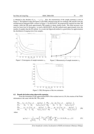
4.2. Efficiency and convergence of sample moments of the EE method
To illustrate the effectiveness and efficiency of the Edgeworth Method, it is mandartory to demosntrate
the convergence of its sample moments as the number of samples P increases [23, 24], and therein compare
it with the Gaussian Kernel. Using the Nakagami Distributed random variables as seen in Figure 1, the true
moments γw of a ND (m = 1, Ω = 1) is compared with sample moments αw [23] for different number of
samples and moment orders w = 1, . . . , 4. The deviation ˆew of the sample moments from the true moment
Int J Elec & Comp Eng, Vol. 10, No. 5, October 2020 : 5535 – 5545

7. Int J Elec & Comp Eng ISSN: 2088-8708 Ì 5541
is obtained as the absolute of (αw − γw)/γw. Also, the monotonicity of the sample moments is seen in
Figure 2. The Kulback Leiber Divergence of the PDFs obtained using the two methods (GK and EE) from the
true/theoretical Nakagami PDF is shown in Figure 3. For KLD=0.01, the proposed EE required less than 300
samples, while the GK needs approximately 500 samples to obtain similar results. This delta increases even
more for lower level of divergency: to reach a KLD=0.0075, the GK method needs approximately twice the
number of samples than the EE method. As a result, the Edgeworth method is a good choice for approximation
the distribution of ranging errors from samples.
100 200 300 400 500 600 700 800 900 1000
0
0.05
0.1
0.15
0.2
0.25
Nakagami m = 1, Ω = 1
Errorew
Number of Samples P
w = {1, 2, 3, 4}
Figure 1. Convergence of sample moments αw
1 2 3 4 5 6 7
0
20
40
60
Nakagami m = 1, Ω = 1
Moment:αw
Order: k
True Moments
P=200
P=500
P=1000
Figure 2. Monotonicity of sample moments αw
100 200 300 400 500 600 700 800 900 1000
0
0.005
0.01
0.015
0.02
0.025
0.03
0.035
0.04
0.045
Nakagami m = 1, Ω = 1
Kullback-LeiblerDivergence
Number of Samples P
PDF - GK
PDF - EE
Figure 3. CKL Divergence of the two estimators
4.3. Bounds derivation using edgeworth expansion
From the formulation of the approximated PDF of the residual error in (19), the creation of the Fisher
information is the same with the GK: This yields
∂lkl
∂xk
=
xk − xl
dkl
vkl − µ
σ2
kl
−
gkl(vkl)
σklfvkl
(vkl)
,
∂lkl
∂yk
=
yk − yl
dkl
vkl − µ
σ2
kl
−
gkl(vkl)
σklfvkl
(vkl)
,
∂lkl
∂xl
= −
xk − xl
dkl
vkl − µ
σ2
kl
−
gkl(vkl)
σklfvkl
(vkl)
,
∂lkl
∂yl
= −
yk − yl
dkl
vkl − µ
σ2
kl
−
gkl(vkl)
σklfvkl
(vkl)
(20)
where
gkl(vkl) =
1
2πσ2
ij
exp −
(vij − µ)2
2σ2
ij
∞
s=1
σs
{km}
(s + 2r)AsHes+2r−1(ˆx) (21)
Error bounds for wireless localization in NLOS environments (Omotayo Oshiga)

8. 5542 Ì ISSN: 2088-8708
The elements of the Fisher Information are similar with the GK except for the coefficient:
Akl = E
vkl − µ
σ2
kl
−
gkl(vkl)
σklfvkl
(vkl)
2
=
∞
−∞
vkl − µ
σ2
kl
−
gkl(vkl)
σklfvkl
(vkl)
2
fvkl
(vkl)dvkl (22)
5. PERFORMANCE EVALUATION
Moving forward from the various theoretical analyses presented in this paper, we can state that the EE
methods can approximate the statistics of ranging errors (using Nakagami Distribution), with lesser samples
and more accuracy with respect to the GK as such we now consider real network topologies to further illustrate
the performances of both methods. Therefore, a region of 10m × 10m is employed, where three (an = 3)
anchors are placed to form a triangular shape and three (n = 3) blindfolded devices (targets), not connected
together, are randomly placed within the convex of the anchors. The two error bounds - the CRLB and the PEB
- will be ultilized to evaluate the performance of the two estimators - EE and GK. The average CRLB for any
network topology can be computed using
¯ε =
1
n
{J−1
} (23)
while the PEB can be illustrated by the 95% Confidence Interval Ci = 0.95, whose mathematical formulation
is shown. The Fisher Ellipse parameters of the i-th target θi are estimated from the covariance matrix Ωθi
,
which is a combination of the error variance σ2
i:x and σ2
i:y on the “x” and “y” dimensions, respectively and the
cross-term σi:xy, given as
Ωθi
σ2
i:x σi:xy
σi:xy σ2
i:y
(24)
The directions of the scattering in the space for the vector θi are known to be directly proportional to the
eigenvalues associated to Ωθi
up to a factor of κi[25, 11, 12]. In particular, the axis direction of the ellipse
which describes this scattering in the space is 2
√
κiλi:1, 2
√
κiλi:2, where
λi:1
1
2
σ2
i:x + σ2
i:y + (σ2
i:x − σ2
i:y)2 + 4σ2
i:xy , λi:2
1
2
σ2
i:x + σ2
i:y − (σ2
i:x − σ2
i:y)2 + 4σ2
i:xy (25)
If σi:y > σi:x, then in (25) the orders of λi:1 and λi:2 are swapped. The proportionality factor κi can be related
to the confidence interval Ci in that the target θi is enclosed in an ellipse, as such κi = −2 ln(1 − Ci)
It follows that the Fisher Ellipse for the i-th target θi is described through the following in [25]
[(x − pi:x) cos γi + (y − pi:y) sin γi]
2
κi · λi:1
+
[(x − pi:x) sin γi − (y − pi:y) cos γi]
2
κi · λi:2
= 1 (26)
where the rotation angle γi describes the offset between the principal axis for the ellipse and reference axis
and it is defined as γi
1
2 arctan
2σi:xy
σ2
i:x − σ2
i:y
– Note that for σ2
i:x = σ2
i:y, then γi = 0.
Figure 4 depicts the level of accuracy and efficiency of the approximated CRLBs ¯ε, as a function of
the sample number P using Nakagami distributed random variables with bij uniformly selected between 0 − 4
for NLOS and σ = 0.5 for both LOS and NLOS ranging errors within each target-to-anchor links.
Int J Elec & Comp Eng, Vol. 10, No. 5, October 2020 : 5535 – 5545

9. Int J Elec & Comp Eng ISSN: 2088-8708 Ì 5543
0 100 200 300 400 500 600 700 800 900 1000
0.08
0.1
0.12
0.14
AverageCRLB¯ε(inmetres)
Number of Samples P
CRLB - GK
CRLB - EE
Theoretical CRLB
Figure 4. Average CRLB as a function of samples
To compare both estimators, a line representing the theoretical CRLB, i.e. computed with perfect
knowledge of the statistic of the propagation channel has been added to the plots. Clearly the CRLB of recon-
structed EE is much closer to the theoretical one than the GK: the EE performs better for any samples. From the
above derived CRLBs, the minimum number of samples P required for obtaining accurate results are analyzed.
As shown in Figure 3, it is seen that the non-parametric estimators converges to the true PDF with sufficient
sample size, therefore the estimated CRLBs converges quickly to a stable value as P increases.
Furthermore, the two estimators are now represented by their respective Fisher ellipses (theoretical
and reconstructed from the two methods) for P = 50 samples as seen in Figure 5. Clearly, the samples
reconstructed with the EE estimator almost perfectly match the theoretical one, where they vary only in the
axis orientation. As the sample number increases to P = 250 samples, the Fisher ellipses of the two estimators
have almost or matching axis orientation to the theoretical PEB with the EE method much closer than the GK
method. To clearly and better capture the differences between the two estimators with respect to the theoretical
PEB, Figure 6 depicts, as a function of the number of samples, the inner product PEB ∆
1
Nt
Nt
i=1
ˆAi · Ai
ˆAiAi
,
where · denotes the inner product, A is the area of the theoretical Fisher ellipse and ˆA is the area of the
reconstructed methods (EE or GK method). From the discussion in this section, it can be clearly seen that
Edgeworth Expansion method performs far better than the Gaussian Kernel method, which therein implies
that theapproximated Fisher Ellipses of Edgeworth Expansion are much closer in size and orientation to the
theoretical Fisher Ellipses.
2 3 4 5 6 7 8 9
0
1
2
3
4
5
6
7
8
9
10
Nakagami b = [0 − 4], σ = 0.5, P = 50
y-coordinates(inmetres)
x-coordinates (in metres)
Anchors
Targets
Theoretical PEB
PEB with EE
PEB with GK
2 3 4 5 6 7 8 9
0
1
2
3
4
5
6
7
8
9
10
Nakagami b = [0 − 4], σ = 0.5, P = 250
y-coordinates(inmetres)
x-coordinates (in metres)
Anchors
Targets
Theoretical CRLB
PEB - EE
PEB - GK
Figure 5. The 95% Fisher ellipses, theoretical, and estimated with P = 50 & 250 samples collected per link
Error bounds for wireless localization in NLOS environments (Omotayo Oshiga)

10. 5544 Ì ISSN: 2088-8708
50 100 150 200 250 300 350 400 450 500
0.72
0.74
0.76
0.78
0.8
0.82
0.84
0.86
Nakagami b = [0 − 4], σ = 0.5
∆M
Number of Samples P
CRLB - GK
CRLB - EE
Figure 6. ∆ as a function of the number of samples
6. CONCLUSIONS
This article clealry focuses on the error analyses of approximating and reconstructing the statistics of
the ranging measurements without a priori knowledge of the wireless channel. A popular and non-paremetric
estimator, the Gaussian kernel was first decribed and utilized for the approximation and reconstruction of the
error distributions from samples and the corresponding error bound was derived. Futhermore, an Edgeworth
Expansion method was therein, to reconstruct the error distribution statistics from samples of the ranging mea-
surements by exploiting the efficiency and effectiveness of moment convergence. This approach was clearly
shown and proven to be valid for Non-Line-of-Sight conditions, where it is impossible to estimate the statistics
of the ranging errors a prior. Results and figures illustrated showed that the Edgeworth expansion technique
is a far more efficient and accurate technique than the Gaussian kernel method, requiring lesser sample size to
reach the samilar level accuracy.
REFERENCES
[1] D. Macagnano, G. Destino, and G. Abreu, ”A comprehensive tutorial on localization: algorithms and
performance analysis tools,” International Journal of Wireless Information Networks, vol. 19, no. 4,
pp. 290-314, 2012.
[2] G. Yanying, A. Lo, and I. Niemegeers, ”A survey of indoor positioning systems for wireless personal
networks,” IEEE Communications Surveys Tutorials, vol. 11, no. 1, pp. 13-32, 2009.
[3] L. Hui, H. Darabi, P. Banerjee, and L. Jing, ”Survey of wireless indoor positioning techniques and sys-
tems,” IEEE Trans. on Systems, Man, and Cybernetics, Part C: Applications and Reviews, vol. 37, no. 6,
pp. 1067-1080, 2007.
[4] N. Patwari, J. Ash, S. Kyperountas, et al, ”Locating the nodes: Cooperative localization in wireless sensor
networks,” IEEE Signal Processing Magazine, vol. 22, no. 4, pp. 54-69, 2005.
[5] K.-T. Feng, C.-L. Chen, and C.-H. Chen, ”Gale: An enhanced geometry-assisted location estimation
algorithm for nlos environments,”IEEE Trans. on Mobile Computing, vol. 7, no. 2, pp. 199-213, 2008.
[6] Y. Qi and H. Kobayashi, ”On geolocation accuracy with prior information in non-line-of-sight environ-
ment,” IEEE Proceedings on the 56th Vehicular Technology Conference-Fall, vol. 1, pp. 285-288, 2002.
[7] H. V. Poor, ”An introduction to signal detection and estimation 2nd Ed,” Springer-Verlag New York, 1994.
[8] H. Van Trees, ”Detection, Estimation, and Modulation Theory,” Wiley, 2004.
[9] S. Kay, ”Fundamentals Statistical Processg,” Prentice Hall, 2001.
[10] T. Wang, ”Cramer-rao bound for localization with a priori knowledge on biased range measurements,”
Aerospace and Electronic Systems, IEEE Transactions on, vol. 48, no. 1, pp. 468-476, 2012.
[11] S. Severi, G. Abreu, G. Destino, and D. Dardari, ”Efficient and Accurate Localization in Multihop Net-
works,” Proc. Asilomar Conf. Signals, Systems, and Computers, 2009.
[12] J. Saloranta, S. Severi, D. Macagnano, and G. Abreu, ”Algebraic confidence for sensor localization,”
Proc. Asilomar Conf. Signals, Systems, and Computers, 2012.
Int J Elec & Comp Eng, Vol. 10, No. 5, October 2020 : 5535 – 5545

11. Int J Elec & Comp Eng ISSN: 2088-8708 Ì 5545
[13] Eric Weisstein, ”Nakagami distribution,” [Online], Avaible: http://mathworld.wolfram.com/
NakaDistribution.html, 2020.
[14] N. Patwari, A. O. Hero, M. Perkins, N. S. Correal, and R. J. O’Dea, ”Relative location estimation in
wireless sensor networks,” IEEE Transactions on Signal Processing, vol. 51, no. 8, pp. 2137-2148, 2003.
[15] H. Miao, K. Yu, and M. J. Juntti, ”Positioning for nlos propagation: Algorithm derivations and cramer-rao
bounds,” IEEE Transactions on Vehicular Technology, vol. 56, no. 5, pp. 2568-2580, 2007.
[16] P. H. Tseng and K. T. Feng, ”Geometry-assisted localization algorithms for wireless networks,”
IEEE Transactions on Mobile Computing, vol. 12, no. 4, pp. 774-789, 2013.
[17] J. Prieto, A. Bahillo, et al, ”Nlos mitigation based on range estimation error characterization in an rtt-
based IEEE 802.11, indoor location,” IEEE International Symposium on Intelligent Signal Processing,
pp. 61-66, 2009.
[18] J. Huang and Q. Wan, ”The crlb for wsns location estimation in nlos environments,” International Con-
ference on Communications, Circuits and Systems, pp. 83-86, 2010.
[19] S. Blinnikov and R. Moessner, ”Expansions for nearly gaussian distributions,” Astronomy and Astro-
physics Supplement Series, vol. 130, pp. 193-205, 1998.
[20] D. Jourdan, J. Deyst, J.J., M. Win, and N. Roy, ”Monte carlo localization in dense multipath environments
using uwb ranging,” IEEE International Conference on Ultra-Wideband, pp. 314-319, 2005.
[21] G.L. St¨uber, ”Principles of Mobile Communication,” Springer Publishing Company, Incorporated, 2011.
[22] J. D. Parson, ”The Mobile Radio Propagation Channel,” Wiley, 2000.
[23] C. Bourin and P. Bondon, ”Efficiency of high-order moment estimates,” IEEE Transactions on Signal
Processing, vol. 46, no. 1, pp. 255-258, 1998.
[24] G. de Abreu, ”Cth16-4: Accurate simulation of piecewise continuous arbitrary nakagami-m phasor pro-
cesses,” IEEE Global Telecommunications Conference, pp. 1-6, 2006.
[25] D. Torrieri, ”Statistical theory of passive location systems,” IEEE Transactions on Aerospace and Elec-
tronic Systems, vol. AES-20, no. 2, pp. 183-198, 1984.
BIOGRAPHIES OF AUTHORS
Omotayo Oshiga received his B.Tech degree in Physics and Telecommunications from the Federal
University of Technology, Minna, Nigeria in 2010 and the M.Sc degree in Wireless Communication
Systems from Brunel University, London, UK in 2011. He received his Ph.D degree in Electrical
Engineering from Jacobs University, Bremen, Germany in February, 2015. He is currently a Senior
Lecturer in the deaprtment of Electrical/Electronics Engineering at the Nile University of Nigeria,
in Abuja, Nigeria. His research interest include various topics in wireless communication and ap-
plied mathematics such as estimation theory, signal processing, wireless communication systems,
positioning, tracking and navigation, wireless sensing etc.
Ali Nyangwarimam Obadiah received his Bachelor of Engineering (B.Eng.) in Electrical and Com-
puter Engineering from the Federal university of Technology Minna, Niger state, Nigeria in 2010 and
a Master of Engineering (M.Eng.) in Electrical-Electronics and Telecommunication Engineering
from the University of Technology Malaysia in 2014. He received a PhD in Electrical Engineer-
ing from University of Technology Malaysia in 2018. He was with the Advanced RF and Microwave
Research Group. He is now a Lecturer with the Department of Computer Engineering, Faculty of En-
gineering, Nile University of Nigeria, Abuja, Nigeria. His research interest includes Radio frequency
devices, reconfigurable antennas, filters and filter-antennas.
Error bounds for wireless localization in NLOS environments (Omotayo Oshiga)