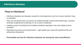
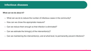
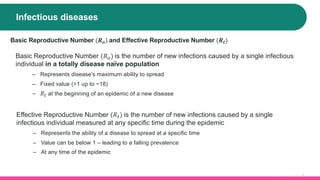
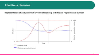
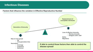
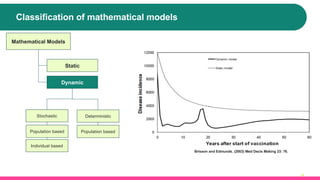
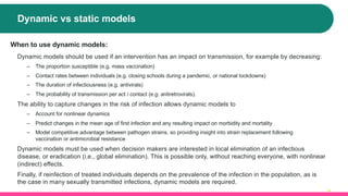
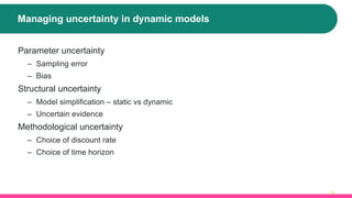
Copyright 2022. All Rights Reserved. Contact Presenter for Permission
An Introduction to Infectious
Disease Modeling
Richard Pitman, PhD
Lead Health Economist & Epidemiologist
Global HEOR & Epidemiology
ICON
Marija Zivkovic-Gojovic, PhD
Senior Consultant
Global HEOR & Epidemiology
ICON
Pragya Khurana, MPH, BS
Epidemiologist
Global HEOR & Epidemiology
ICON
Infectious Diseases
Infectious diseases
So why are
infectious
diseases
important?
Infectious diseases
4
They’re infectious!
‒ Infectious diseases are diseases caused by microorganisms such as viruses, bacteria, fungi
or parasites.
‒ They can be spread from one person to another through contact with bodily fluids, aerosols
(through coughing and sneezing), or via a vector (mosquito).
‒ Leading cause of morbidity and mortality worldwide specially in low and middle-income
countries
‒ Significant economic and social burden – high health-care costs with significant life and
productivity disruptions
‒ Preventable services for infectious diseases are among the most cost-effective.
Infectious diseases
5
What can we do about it?
‒ What can we do to reduce the number of infectious cases in the community?
‒ How can we chose the appropriate measure?
‒ Can we reduce them enough so that infection is eliminated?
‒ Can we estimate the timing(s) of the intervention(s)?
‒ Can we maintaining the intervention(s), and at what level, to permanently prevent infections?
Infectious diseases
6
Basic Reproductive Number (𝑹𝒐) and Effective Reproductive Number (𝑹𝒕)
Basic Reproductive Number (𝑅!) is the number of new infections caused by a single infectious
individual in a totally disease naïve population
‒ Represents disease’s maximum ability to spread
‒ Fixed value (>1 up to ~18)
‒ 𝑅# at the beginning of an epidemic of a new disease
Effective Reproductive Number (𝑅") is the number of new infections caused by a single
infectious individual measured at any specific time during the epidemic
‒ Represents the ability of a disease to spread at a specific time
‒ Value can be below 1 – leading to a falling prevalence
‒ At any time of the epidemic
Infectious diseases
7
Representation of an Epidemic Curve in relationship to Effective Reproductive Number
Time
Infections
0
= R0
Epidemic curve
Effective
reproductive
number
0
2
1
Effective reproductive number
Infectious Diseases
8
Replenishment of
susceptible individuals
Generation of Immunity
Rate of viral spread
‒ R0
‒ Viral generation time
Vaccination
‒ Coverage
‒ Frequency
‒ Behaviour
Loss of effective immunity
‒ Waning immunity
‒ Antigenic drift / shift
Births
Migrations
Factors that influence the variation in Effective Reproductive Number
𝑹𝒕
Generation of Immunity
If able to control those factors then able to control the
disease spread!
Dynamic Transmission Models
Infectious Disease Modelling
Mathematical modelling
10
Mathematical modelling is the process of creating a mathematical representation of a real-
world problem to make a prediction, provide insight and potentially find solutions.
What is mathematical modelling?
Real-World
Problem
Mathematical representation
Real-World
Solution
Variables +
Parameters
Modelling Mechanism Results
Calibration Process.
Scenario Analysis
Outputs
Inputs
Data
Mathematical modelling
11
Why mathematical modelling?
‒ Provides a framework for understanding and discussion, with explicit assumptions
‒ Allows us to transparently account for uncertainty
‒ Can provide insights into solutions to problems / options to chose from (multiple scenarios)
‒ Can give answers to complex questions that otherwise can not be established
‒ Are a means to evaluate the efficiency, effectiveness, value and impact of any health
related services through the use of Health-Economic Analysis
Classification of mathematical models
12
Mathematical Models
Static
Dynamic
Stochastic Deterministic
Population based
Individual based
Population based
Brisson and Edmunds. (2003) Med Decis Making 23: 76.
Dynamic vs static models
13
When to use static models:
‒ A static model is acceptable if the intervention has no impact on disease transmission
‒ Static models may be acceptable, as an initial approximation, when their projections
suggest that an intervention is cost-effective, and dynamic effects would further enhance this
(e.g., via prevention of secondary cases)
‒ Adopting such an approach is risky, as it assumes that dynamic effects will always enhance
cost-effectiveness. This is NOT always the case
‒ Ignoring dynamic effects, so incorrectly valuing an intervention, can lead to poor public health
decision making if policymakers use such estimates to decide on the optimum allocation of a
limited health care budget
Dynamic vs static models
14
When to use dynamic models:
Dynamic models should be used if an intervention has an impact on transmission, for example by decreasing:
‒ The proportion susceptible (e.g. mass vaccination)
‒ Contact rates between individuals (e.g. closing schools during a pandemic, or national lockdowns)
‒ The duration of infectiousness (e.g. antivirals)
‒ The probability of transmission per act / contact (e.g. antiretrovirals).
The ability to capture changes in the risk of infection allows dynamic models to
‒ Account for nonlinear dynamics
‒ Predict changes in the mean age of first infection and any resulting impact on morbidity and mortality
‒ Model competitive advantage between pathogen strains, so providing insight into strain replacement following
vaccination or antimicrobial resistance
Dynamic models must be used when decision makers are interested in local elimination of an infectious
disease, or eradication (i.e., global elimination). This is possible only, without reaching everyone, with nonlinear
(indirect) effects.
Finally, if reinfection of treated individuals depends on the prevalence of the infection in the population, as is
the case in many sexually transmitted infections, dynamic models are required.
Managing uncertainty in dynamic models
15
Parameter uncertainty
‒ Sampling error
‒ Bias
Structural uncertainty
‒ Model simplification – static vs dynamic
‒ Uncertain evidence
Methodological uncertainty
‒ Choice of discount rate
‒ Choice of time horizon
16
Parameter uncertainty - Probabilistic sensitivity analysis
Input variable 1
Input variable 3
Input variable 2
Number
of
samples
Outcome variable
Repeatedly sample
joint distribution
95% uncertainty interval
Case Study:
Development of a dynamic
transmission/cost effectiveness model
for influenza A and B
R.J. Pitman, L.J. White & M.J. Sculpher (2012) Vaccine 30: 1202 - 1218
R.J. Pitman, L.D. Nagy & M.J. Sculpher (2013) Vaccine 31: 927 - 942
Background & Objectives
18
Economic modelling of childhood influenza vaccination
Objectives
‒ To create a childhood influenza A/B economic model that incorporates dynamic transmission and indirect
effects
‒ To examine the cost-effectiveness of an investigational influenza vaccine, LAIV for children in the United
Kingdom
19
Methods
Infectious model state is the link to the CE
module
Estimates of UK influenza burden
UK ‘influenza like illness’ data
Basic construct of cost-effectiveness model
CPRD HES ONS
20
Linking influenza incidence to costs and outcomes
Influenza attributable resource use/costs and mortality are key
‒ UK databases – Influenza-like-illness (ILI)
attributed GP visits/medication (GPRD),
hospitalization (HES) and mortality (ONS),
laboratory confirmed infection data (LabBase)
‒ Multiple regression analysis to estimate the
influenza attributable proportion of ILI attributed
outcomes
‒ Simulated age-stratified incidence of influenza
A/B combined with regression analysis of burden
to produce probabilities of an incident influenza
infection leading to a GP consultation,
Hospitalization or death
‒ Costs and LY decrements based on estimates
from 2003 HTA report (costs inflated to 2009
prices)
21
Model assumptions
The following vaccination scenarios were considered, for the target vaccine and a comparator vaccine:
‒ 10% coverage in 2 – 18
‒ 50% coverage in 2 – 18
‒ 80% coverage in 2 – 18
‒ 80% coverage in 2 – 4
Vaccination scenario
22
Key parameters
‒ Who Acquires Infection From Whom (WAIFW) matrix
‒ Transmission coefficient
‒ Duration of
‒ Latency, 2 days
‒ Infectiousness, 2 days
‒ Immunity, Influenza A: 6 years, B: 12 years
‒ Basic reproductive rate (Ro) of 1.8
‒ Discount rate 3.5%
‒ Time horizon 15 years
23
Results
0
200,000
400,000
600,000
800,000
1,000,000
1,200,000
1,400,000
1,600,000
1,800,000
2,000,000
Influenza A Influenza B Influenza A Influenza B Influenza A Influenza B Influenza A Influenza B
Cases averted Cases averted Cases averted Cases averted
LAIV 10% coverage 2 - 18 year
olds
LAIV 50% coverage 2 - 18 year
olds
LAIV80% coverage 2 - 18 year
olds
LAIV 80% coverage 2 - 4 year
olds
0 - 11 mo
12 - 23 mo
24 - 59 mo
5 - 10 yr
11 - 18 yr
19 - 49 yr
50 - 64 yr
65+ yr
Averted infectious influenza cases
Results: Exploratory model behaviour in CE plane
24
Results: Exploratory model behaviour in CE plane
25
80% vaccination 2-18 yrs
50% vaccination 2-18 yrs
10% vaccination 2-18 yrs
80% vaccination 2-4 yrs
80% vaccination 2-18 yrs
excluding herd immunity effects
-1,000
0
1,000
2,000
3,000
4,000
5,000
6,000
7,000
0.0 0.5 1.0 1.5 2.0 2.5 3.0 3.5 4.0 4.5 5.0
Incremental QALYs
incremental
cost
(£)
Indirect protection
65+ age group: 75% vaccination
QALYs: Turner D. et al
Health Technol
Assess. 2003;
7: 1-170
Costing: Ibid.
Time frame: 15yr cumulative
Results: Choosing the optimum strategy
26
Cost-effectiveness acceptability curve Cost-effectiveness acceptability frontier
Conclusions
27
– Accounting for indirect effects significantly increased the estimated cost-effectiveness
of the vaccine, relative to static cost-effectiveness models
– Dynamic transmission modelling allowed us to accurately estimate and compare the
value of multiple vaccine strategies, while accounting for the impact of parameter and
structural uncertainty
Final Remarks
Advantages of dynamic transmission models
29
Dynamic
Transmission
Models
Powerful
tool that can be used to
investigate, research and
explore complex systems
Sophisticated
framework able to capture
mechanism other models
cannot (indirect effects /
herd immunity)
Comprehensive
More accurately capture the
critical drivers of the value
of interventions
Uncertainty
Appropriately account for
the impact of uncertainty in
a non-linear system
Versatile
application
an important component in
health–economic analysis
Applications: Real-world evidence
30
Estimate
burden of
the disease
Vaccine
policy
analysis
Evaluate cost-
effectiveness
and budget
impact of
vaccination
programmes
Evaluate
different
mitigation
strategies
31
Resources
Media article: A challenge of
pandemic proportions
Media article: Will COVID-
19 bring lasting change in
clinical trial practices?
Whitepaper: Antimicrobial
resistance
Whitepaper: The evolution
of HIV treatments
Whitepaper: Pandemic
respiratory vaccine clinical
trials
ICON Infectious Diseases Insights: Whitepapers, blogs, articles
ICONplc.com
© 2022 ICON. All rights reserved.
Thank you for participating!
CLICK HERE to learn more and
watch the webinar

An Introduction to Infectious Disease Modeling

  • 1.
    Copyright 2022. AllRights Reserved. Contact Presenter for Permission An Introduction to Infectious Disease Modeling Richard Pitman, PhD Lead Health Economist & Epidemiologist Global HEOR & Epidemiology ICON Marija Zivkovic-Gojovic, PhD Senior Consultant Global HEOR & Epidemiology ICON Pragya Khurana, MPH, BS Epidemiologist Global HEOR & Epidemiology ICON
  • 2.
  • 3.
    Infectious diseases So whyare infectious diseases important?
  • 4.
    Infectious diseases 4 They’re infectious! ‒Infectious diseases are diseases caused by microorganisms such as viruses, bacteria, fungi or parasites. ‒ They can be spread from one person to another through contact with bodily fluids, aerosols (through coughing and sneezing), or via a vector (mosquito). ‒ Leading cause of morbidity and mortality worldwide specially in low and middle-income countries ‒ Significant economic and social burden – high health-care costs with significant life and productivity disruptions ‒ Preventable services for infectious diseases are among the most cost-effective.
  • 5.
    Infectious diseases 5 What canwe do about it? ‒ What can we do to reduce the number of infectious cases in the community? ‒ How can we chose the appropriate measure? ‒ Can we reduce them enough so that infection is eliminated? ‒ Can we estimate the timing(s) of the intervention(s)? ‒ Can we maintaining the intervention(s), and at what level, to permanently prevent infections?
  • 6.
    Infectious diseases 6 Basic ReproductiveNumber (𝑹𝒐) and Effective Reproductive Number (𝑹𝒕) Basic Reproductive Number (𝑅!) is the number of new infections caused by a single infectious individual in a totally disease naïve population ‒ Represents disease’s maximum ability to spread ‒ Fixed value (>1 up to ~18) ‒ 𝑅# at the beginning of an epidemic of a new disease Effective Reproductive Number (𝑅") is the number of new infections caused by a single infectious individual measured at any specific time during the epidemic ‒ Represents the ability of a disease to spread at a specific time ‒ Value can be below 1 – leading to a falling prevalence ‒ At any time of the epidemic
  • 7.
    Infectious diseases 7 Representation ofan Epidemic Curve in relationship to Effective Reproductive Number Time Infections 0 = R0 Epidemic curve Effective reproductive number 0 2 1 Effective reproductive number
  • 8.
    Infectious Diseases 8 Replenishment of susceptibleindividuals Generation of Immunity Rate of viral spread ‒ R0 ‒ Viral generation time Vaccination ‒ Coverage ‒ Frequency ‒ Behaviour Loss of effective immunity ‒ Waning immunity ‒ Antigenic drift / shift Births Migrations Factors that influence the variation in Effective Reproductive Number 𝑹𝒕 Generation of Immunity If able to control those factors then able to control the disease spread!
  • 9.
  • 10.
    Mathematical modelling 10 Mathematical modellingis the process of creating a mathematical representation of a real- world problem to make a prediction, provide insight and potentially find solutions. What is mathematical modelling? Real-World Problem Mathematical representation Real-World Solution Variables + Parameters Modelling Mechanism Results Calibration Process. Scenario Analysis Outputs Inputs Data
  • 11.
    Mathematical modelling 11 Why mathematicalmodelling? ‒ Provides a framework for understanding and discussion, with explicit assumptions ‒ Allows us to transparently account for uncertainty ‒ Can provide insights into solutions to problems / options to chose from (multiple scenarios) ‒ Can give answers to complex questions that otherwise can not be established ‒ Are a means to evaluate the efficiency, effectiveness, value and impact of any health related services through the use of Health-Economic Analysis
  • 12.
    Classification of mathematicalmodels 12 Mathematical Models Static Dynamic Stochastic Deterministic Population based Individual based Population based Brisson and Edmunds. (2003) Med Decis Making 23: 76.
  • 13.
    Dynamic vs staticmodels 13 When to use static models: ‒ A static model is acceptable if the intervention has no impact on disease transmission ‒ Static models may be acceptable, as an initial approximation, when their projections suggest that an intervention is cost-effective, and dynamic effects would further enhance this (e.g., via prevention of secondary cases) ‒ Adopting such an approach is risky, as it assumes that dynamic effects will always enhance cost-effectiveness. This is NOT always the case ‒ Ignoring dynamic effects, so incorrectly valuing an intervention, can lead to poor public health decision making if policymakers use such estimates to decide on the optimum allocation of a limited health care budget
  • 14.
    Dynamic vs staticmodels 14 When to use dynamic models: Dynamic models should be used if an intervention has an impact on transmission, for example by decreasing: ‒ The proportion susceptible (e.g. mass vaccination) ‒ Contact rates between individuals (e.g. closing schools during a pandemic, or national lockdowns) ‒ The duration of infectiousness (e.g. antivirals) ‒ The probability of transmission per act / contact (e.g. antiretrovirals). The ability to capture changes in the risk of infection allows dynamic models to ‒ Account for nonlinear dynamics ‒ Predict changes in the mean age of first infection and any resulting impact on morbidity and mortality ‒ Model competitive advantage between pathogen strains, so providing insight into strain replacement following vaccination or antimicrobial resistance Dynamic models must be used when decision makers are interested in local elimination of an infectious disease, or eradication (i.e., global elimination). This is possible only, without reaching everyone, with nonlinear (indirect) effects. Finally, if reinfection of treated individuals depends on the prevalence of the infection in the population, as is the case in many sexually transmitted infections, dynamic models are required.
  • 15.
    Managing uncertainty indynamic models 15 Parameter uncertainty ‒ Sampling error ‒ Bias Structural uncertainty ‒ Model simplification – static vs dynamic ‒ Uncertain evidence Methodological uncertainty ‒ Choice of discount rate ‒ Choice of time horizon
  • 16.
    16 Parameter uncertainty -Probabilistic sensitivity analysis Input variable 1 Input variable 3 Input variable 2 Number of samples Outcome variable Repeatedly sample joint distribution 95% uncertainty interval
  • 17.
    Case Study: Development ofa dynamic transmission/cost effectiveness model for influenza A and B R.J. Pitman, L.J. White & M.J. Sculpher (2012) Vaccine 30: 1202 - 1218 R.J. Pitman, L.D. Nagy & M.J. Sculpher (2013) Vaccine 31: 927 - 942
  • 18.
    Background & Objectives 18 Economicmodelling of childhood influenza vaccination Objectives ‒ To create a childhood influenza A/B economic model that incorporates dynamic transmission and indirect effects ‒ To examine the cost-effectiveness of an investigational influenza vaccine, LAIV for children in the United Kingdom
  • 19.
    19 Methods Infectious model stateis the link to the CE module Estimates of UK influenza burden UK ‘influenza like illness’ data Basic construct of cost-effectiveness model CPRD HES ONS
  • 20.
    20 Linking influenza incidenceto costs and outcomes Influenza attributable resource use/costs and mortality are key ‒ UK databases – Influenza-like-illness (ILI) attributed GP visits/medication (GPRD), hospitalization (HES) and mortality (ONS), laboratory confirmed infection data (LabBase) ‒ Multiple regression analysis to estimate the influenza attributable proportion of ILI attributed outcomes ‒ Simulated age-stratified incidence of influenza A/B combined with regression analysis of burden to produce probabilities of an incident influenza infection leading to a GP consultation, Hospitalization or death ‒ Costs and LY decrements based on estimates from 2003 HTA report (costs inflated to 2009 prices)
  • 21.
    21 Model assumptions The followingvaccination scenarios were considered, for the target vaccine and a comparator vaccine: ‒ 10% coverage in 2 – 18 ‒ 50% coverage in 2 – 18 ‒ 80% coverage in 2 – 18 ‒ 80% coverage in 2 – 4 Vaccination scenario
  • 22.
    22 Key parameters ‒ WhoAcquires Infection From Whom (WAIFW) matrix ‒ Transmission coefficient ‒ Duration of ‒ Latency, 2 days ‒ Infectiousness, 2 days ‒ Immunity, Influenza A: 6 years, B: 12 years ‒ Basic reproductive rate (Ro) of 1.8 ‒ Discount rate 3.5% ‒ Time horizon 15 years
  • 23.
    23 Results 0 200,000 400,000 600,000 800,000 1,000,000 1,200,000 1,400,000 1,600,000 1,800,000 2,000,000 Influenza A InfluenzaB Influenza A Influenza B Influenza A Influenza B Influenza A Influenza B Cases averted Cases averted Cases averted Cases averted LAIV 10% coverage 2 - 18 year olds LAIV 50% coverage 2 - 18 year olds LAIV80% coverage 2 - 18 year olds LAIV 80% coverage 2 - 4 year olds 0 - 11 mo 12 - 23 mo 24 - 59 mo 5 - 10 yr 11 - 18 yr 19 - 49 yr 50 - 64 yr 65+ yr Averted infectious influenza cases
  • 24.
    Results: Exploratory modelbehaviour in CE plane 24
  • 25.
    Results: Exploratory modelbehaviour in CE plane 25 80% vaccination 2-18 yrs 50% vaccination 2-18 yrs 10% vaccination 2-18 yrs 80% vaccination 2-4 yrs 80% vaccination 2-18 yrs excluding herd immunity effects -1,000 0 1,000 2,000 3,000 4,000 5,000 6,000 7,000 0.0 0.5 1.0 1.5 2.0 2.5 3.0 3.5 4.0 4.5 5.0 Incremental QALYs incremental cost (£) Indirect protection 65+ age group: 75% vaccination QALYs: Turner D. et al Health Technol Assess. 2003; 7: 1-170 Costing: Ibid. Time frame: 15yr cumulative
  • 26.
    Results: Choosing theoptimum strategy 26 Cost-effectiveness acceptability curve Cost-effectiveness acceptability frontier
  • 27.
    Conclusions 27 – Accounting forindirect effects significantly increased the estimated cost-effectiveness of the vaccine, relative to static cost-effectiveness models – Dynamic transmission modelling allowed us to accurately estimate and compare the value of multiple vaccine strategies, while accounting for the impact of parameter and structural uncertainty
  • 28.
  • 29.
    Advantages of dynamictransmission models 29 Dynamic Transmission Models Powerful tool that can be used to investigate, research and explore complex systems Sophisticated framework able to capture mechanism other models cannot (indirect effects / herd immunity) Comprehensive More accurately capture the critical drivers of the value of interventions Uncertainty Appropriately account for the impact of uncertainty in a non-linear system Versatile application an important component in health–economic analysis
  • 30.
    Applications: Real-world evidence 30 Estimate burdenof the disease Vaccine policy analysis Evaluate cost- effectiveness and budget impact of vaccination programmes Evaluate different mitigation strategies
  • 31.
    31 Resources Media article: Achallenge of pandemic proportions Media article: Will COVID- 19 bring lasting change in clinical trial practices? Whitepaper: Antimicrobial resistance Whitepaper: The evolution of HIV treatments Whitepaper: Pandemic respiratory vaccine clinical trials ICON Infectious Diseases Insights: Whitepapers, blogs, articles
  • 32.
    ICONplc.com © 2022 ICON.All rights reserved.
  • 33.
    Thank you forparticipating! CLICK HERE to learn more and watch the webinar