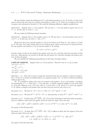
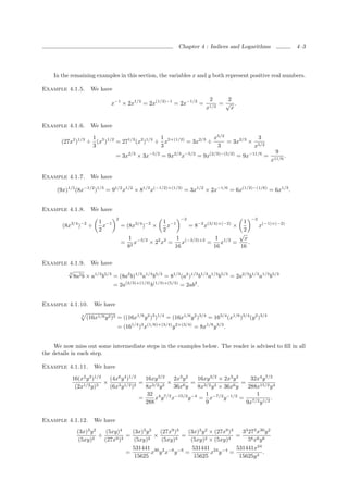
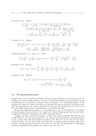
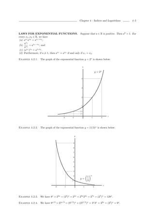
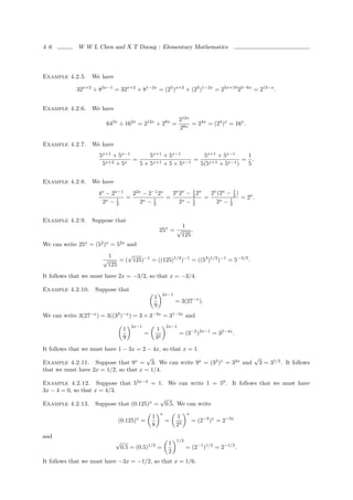
This document provides an overview of indices and logarithms in elementary mathematics. It begins by defining integer indices and establishing laws for integer indices. It then extends the definition of indices to rational numbers by defining qth roots. Laws of indices are generalized to apply to rational exponents. Examples are provided to illustrate working with rational exponents. The chapter then introduces exponential functions, defining them as continuous functions that pass through the points (k, ak) for rational k. Laws for exponential functions are stated for real exponents.

1. ELEMENTARY MATHEMATICS
W W L CHEN and X T DUONG
c W W L Chen, X T Duong and Macquarie University, 1999.
This work is available free, in the hope that it will be useful.
Any part of this work may be reproduced or transmitted in any form or by any means, electronic or mechanical, including
photocopying, recording, or any information storage and retrieval system, with or without permission from the authors.
Chapter 4
INDICES AND LOGARITHMS
4.1. Indices
Given any non-zero real number a ∈ R and any natural number k ∈ N, we often write
ak = a × . . . × a . (1)
k
This definition can be extended to all integers k ∈ Z by writing
a0 = 1 (2)
and
1 1
ak = = (3)
a−k a × ... × a
−k
whenever k is a negative integer, noting that −k ∈ N in this case.
It is not too difficult to establish the following.
LAWS OF INTEGER INDICES. Suppose that a, b ∈ R are non-zero. Then for every m, n ∈ Z,
we have
(a) am an = am+n ;
am
(b) n = am−n ;
a
(c) (am )n = amn ; and
(d) (ab)m = am bm .
† This chapter was written at Macquarie University in 1999.

2. 4–2 W W L Chen and X T Duong : Elementary Mathematics
We now further extend the definition of ak to all rational numbers k ∈ Q. To do this, we first of all
need to discuss the q-th roots of a positive real number a, where q ∈ N. This is an extension of the idea
of square roots discussed in Section 1.2. We recall the following definition, slightly modified here.
Definition. Suppose that a ∈ R is positive. We say that x > 0 is the positive square root of a if
√
x2 = a. In this case, we write x = a.
We now make the following natural extension.
Definition. Suppose that a ∈ R is positive and q ∈ N. We say that x > 0 is the positive q-th root of
√
a if xq = a. In this case, we write x = q a = a1/q .
Recall now that every rational number k ∈ Q can be written in the form k = p/q, where p ∈ Z and
q ∈ N. We may, if we wish, assume that p/q is in lowest terms, where p and q have no common factors.
For any positive real number a ∈ R, we can now define ak by writing
ak = ap/q = (a1/q )p = (ap )1/q . (4)
In other words, we first of all calculate the positive q-th root of a, and then take the p-th power of this
q-th root. Alternatively, we can first of all take the p-th power of a, and then calculate the positive q-th
root of this p-th power.
We can establish the following generalization of the Laws of integer indices.
LAWS OF INDICES. Suppose that a, b ∈ R are positive. Then for every m, n ∈ Q, we have
(a) am an = am+n ;
am
(b) n = am−n ;
a
(c) (am )n = amn ; and
(d) (ab)m = am bm .
Remarks. (1) Note that we have to make the restriction that the real numbers a and b are positive.
If a = 0, then ak is clearly not defined when k is a negative integer. If a < 0, then we will have problems
taking square roots.
(2) It is possible to define cube roots of a negative real number a. It is a real number x satisfying
the requirement x3 = a. Note that x < 0 in this case. A similar argument applies to q-th roots when
q ∈ N is odd. However, if q ∈ N is even, then xq ≥ 0 for every x ∈ R, and so xq = a for any negative
a ∈ R. Hence a negative real number does not have real q-th roots for any even q ∈ N.
Example 4.1.1. We have 24 × 23 = 16 × 8 = 128 = 27 = 24+3 and 2−3 = 1/8.
Example 4.1.2. We have 82/3 = (81/3 )2 = 22 = 4. Alternatively, we have 82/3 = (82 )1/3 = 641/3 = 4.
√ √ √
Example 4.1.3. To show that 5 + 2 6 = 2+ 3, we first of all observe that both sides are positive,
and so it suffices to show that the squares of the two sides are equal. Note now that
√ √ √ √ √ √ √
( 2 + 3)2 = ( 2)2 + 2 2 3 + ( 3)2 = 5 + 2 × 21/2 31/2 = 5 + 2(2 × 3)1/2 = 5 + 2 6,
the square of the left hand side.
√ √ √
Example 4.1.4. To show that 8 − 4 3 = 6 − 2, it suffices to show that the squares of the two
sides are equal. Note now that
√ √ √ √ √ √
( 6 − 2)2 = ( 6)2 − 2 6 2 + ( 2)2 = 8 − 2 × 61/2 21/2 = 8 − 2(6 × 2)1/2
√ √ √
= 8 − 2 12 = 8 − 2 × 2 3 = 8 − 4 3,
the square of the left hand side.

3. Chapter 4 : Indices and Logarithms 4–3
In the remaining examples in this section, the variables x and y both represent positive real numbers.
Example 4.1.5. We have
2 2
x−1 × 2x1/2 = 2x(1/2)−1 = 2x−1/2 = =√ .
x1/2 x
Example 4.1.6. We have
1 1 x5/2 3
(27x2 )1/3 ÷ (x5 )1/2 = 271/3 (x2 )1/3 ÷ x5×(1/2) = 3x2/3 ÷ = 3x2/3 × 5/2
3 3 3 x
9
= 3x2/3 × 3x−5/2 = 9x2/3 x−5/2 = 9x(2/3)−(5/2) = 9x−11/6 = .
x11/6
Example 4.1.7. We have
(9x)1/2 (8x−1/2 )1/3 = 91/2 x1/2 × 81/3 x(−1/2)×(1/3) = 3x1/2 × 2x−1/6 = 6x(1/2)−(1/6) = 6x1/3 .
Example 4.1.8. We have
2 −2 −2
1 −1 1 −1 1
(8x3/4 )−2 ÷ x = (8x3/4 )−2 × x = 8−2 x(3/4)×(−2) × x(−1)×(−2)
2 2 2
√
1 −3/2 1 (−3/2)+2 1 1/2 x
= x × 22 x2 = x = x = .
82 16 16 16
Example 4.1.9. We have
√
8a2 b × a1/3 b5/3 = (8a2 b)1/3 a1/3 b5/3 = 81/3 (a2 )1/3 b1/3 a1/3 b5/3 = 2a2/3 b1/3 a1/3 b5/3
3
= 2a(2/3)+(1/3) b(1/3)+(5/3) = 2ab2 .
Example 4.1.10. We have
4
(16x1/6 y 2 )3 = ((16x1/6 y 2 )3 )1/4 = (16x1/6 y 2 )3/4 = 163/4 (x1/6 )3/4 (y 2 )3/4
= (161/4 )3 x(1/6)×(3/4) y 2×(3/4) = 8x1/8 y 3/2 .
We now miss out some intermediate steps in the examples below. The reader is advised to fill in all
the details in each step.
Example 4.1.11. We have
16(x2 y 3 )1/2 (4x6 y 4 )1/2 16xy 3/2 2x3 y 2 16xy 3/2 × 2x3 y 2 32x4 y 7/2
× = 3/2 3 × = 3/2 3 =
(2x1/2 y)3 (6x3 y 1/2 )2 8x y 36x6 y 8x y × 36x6 y 288x15/2 y 4
32 4 7/2 −15/2 −4 1 −7/2 −1/2 1
= x y x y = x y = 7/2 1/2 .
288 9 9x y
Example 4.1.12. We have
(3x)3 y 2 (5xy)4 (3x)3 y 2 (27x9 )3 (3x)3 y 2 × (27x9 )3 33 273 x30 y 2
2
÷ 9 )3
= 2
× 4
= 2 × (5xy)4
=
(5xy) (27x (5xy) (5xy) (5xy) 56 x6 y 6
531441 30 2 −6 −6 531441 24 −4 531441x24
= x y x y = x y = .
15625 15625 15625y 4

4. 4–4 W W L Chen and X T Duong : Elementary Mathematics
Example 4.1.13. We have
x−1 + y −1 x−1 − y −1 (x − y)(x−1 + y −1 ) − (x−1 − y −1 )(x + y)
− =
x+y x−y (x − y)(x + y)
(1 + xy −1 − yx−1 − 1) − (1 + yx−1 − xy −1 − 1) 2(xy −1 − yx−1 )
= =
(x − y)(x + y) (x − y)(x + y)
2 x y 2 x2 − y 2 2
= × − = × = .
(x − y)(x + y) y x (x − y)(x + y) xy xy
Example 4.1.14. We have
x−1 − y −1 1 1 1 1 y − x y 2 − x2
−2 − y −2
= (x−1 − y −1 ) ÷ (x−2 − y −2 ) = − ÷ 2
− 2 = ÷
x x y x y xy x2 y 2
y−x x2 y 2 x2 y 2 (y − x) x2 y 2 (y − x) xy
= × 2 = = = .
xy y −x 2 xy(y 2 − x2 ) xy(y − x)(y + x) x+y
Alternatively, write a = x−1 and b = y −1 . Then
−1 −1
x−1 − y −1 a−b 1 1 1 x+y xy
−2 − y −2
= 2 = = (a + b)−1 = + = = .
x a −b 2 a+b x y xy x+y
Example 4.1.15. We have
x2 1 1 x2 x+y x2 xy x3
x2 y −1 ÷ (x−1 + y −1 ) = ÷ + = ÷ = × = .
y x y y xy y x+y x+y
Example 4.1.16. We have
−1
1
xy ÷ ((x−1 + y)−1 )−1 = xy × (x−1 + y)−1 = xy × +y
x
−1
1 + xy x x2 y
= xy × = xy × = .
x 1 + xy 1 + xy
4.2. The Exponential Functions
Suppose that a ∈ R is a positive real number. We have shown in Section 4.1 that we can use (1)–(4)
to define ak for every rational number k ∈ Q. Here we shall briefly discuss how we may further extend
the definition of ak to a function ax defined for every real number x ∈ R. A thorough treatment of this
extension will require the study of the theory of continuous functions as well as the well known result
that the rational numbers are “dense” among the real numbers, and is beyond the scope of this set of
notes. We shall instead confine our discussion here to a heuristic treatment.
We all know simple functions like y = x2 (a parabola) or y = 2x + 3 (a straight line). It is possible
to draw the graph of such a function in one single stroke, without lifting our pen from the paper before
completing the drawing. Such functions are called continuous functions.
Suppose now that a positive real number a ∈ R has been chosen and fixed. Note that we have
already defined ak for every rational number k ∈ Q. We now draw the graph of a continuous function
on the xy-plane which will pass through every point (k, ak ) where k ∈ Q. It turns out that such a
function is unique. In other words, there is one and only one continuous function whose graph on the
xy-plane will pass through every point (k, ak ) where k ∈ Q. We call this function the exponential
function corresponding to the positive real number a, and write f (x) = ax .

5. Chapter 4 : Indices and Logarithms 4–5
LAWS FOR EXPONENTIAL FUNCTIONS. Suppose that a ∈ R is positive. Then a0 = 1. For
every x1 , x2 ∈ R, we have
(a) ax1 ax2 = ax1 +x2 ;
ax1
(b) x2 = ax1 −x2 ; and
a
(c) (ax1 )x2 = ax1 x2 .
(d) Furthermore, if a = 1, then ax1 = ax2 if and only if x1 = x2 .
Example 4.2.1. The graph of the exponential function y = 2x is shown below:
y
y = 2x
4
3
2
1
1/2
1/4
x
-2 -1 1 2
Example 4.2.2. The graph of the exponential function y = (1/3)x is shown below:
y
9
8
7
6
5
4
3
2 x
1
y=
1 3
x
-2 -1 1 2
Example 4.2.3. We have 8x × 24x = (23 )x × 24x = 23x 24x = 27x = (27 )x = 128x .
Example 4.2.4. We have 9x/2 × 27x/3 = (91/2 )x × (271/3 )x = 3x 3x = 32x = (32 )x = 9x .

6. 4–6 W W L Chen and X T Duong : Elementary Mathematics
Example 4.2.5. We have
32x+2 ÷ 82x−1 = 32x+2 × 81−2x = (25 )x+2 × (23 )1−2x = 25x+10 23−6x = 213−x .
Example 4.2.6. We have
212x
642x ÷ 162x = 212x ÷ 28x = = 24x = (24 )x = 16x .
28x
Example 4.2.7. We have
5x+1 + 5x−1 5x+1 + 5x−1 5x+1 + 5x−1 1
= = = .
5 x+2 + 5x 5×5 x+1 + 5 × 5x−1 5(5x+1 + 5x−1 ) 5
Example 4.2.8. We have
4x − 2x−1 22x − 2−1 2x 2x 2x − 1 2x 2x (2x − 1 )
= = 2
= 2
= 2x .
2x − 12 2x − 1
2 2x − 1
2 2x − 12
Example 4.2.9. Suppose that
1
25x = √ .
125
We can write 25x = (52 )x = 52x and
1 √
√ = ( 125)−1 = ((125)1/2 )−1 = ((53 )1/2 )−1 = 5−3/2 .
125
It follows that we must have 2x = −3/2, so that x = −3/4.
Example 4.2.10. Suppose that
2x−1
1
= 3(27−x ).
9
We can write 3(27−x ) = 3((33 )−x ) = 3 × 3−3x = 31−3x and
2x−1 2x−1
1 1
= = (3−2 )2x−1 = 32−4x .
9 32
It follows that we must have 1 − 3x = 2 − 4x, so that x = 1.
√ √
Example 4.2.11. Suppose that 9x = 3. We can write 9x = (32 )x = 32x and 3 = 31/2 . It follows
that we must have 2x = 1/2, so that x = 1/4.
Example 4.2.12. Suppose that 53x−4 = 1. We can write 1 = 50 . It follows that we must have
3x − 4 = 0, so that x = 4/3.
√
Example 4.2.13. Suppose that (0.125)x = 0.5. We can write
x x
1 1
(0.125)x = = = (2−3 )x = 2−3x
8 23
and
√ 1
1/2
0.5 = (0.5)1/2 = = (2−1 )1/2 = 2−1/2 .
2
It follows that we must have −3x = −1/2, so that x = 1/6.

7. Chapter 4 : Indices and Logarithms 4–7
Example 4.2.14. Suppose that 81−x × 2x−3 = 4. We can write 4 = 22 and
81−x × 2x−3 = (23 )1−x × 2x−3 = 23−3x × 2x−3 = 2−2x .
It follows that we must have −2x = 2, so that x = −1.
4.3. The Logarithmic Functions
The logarithmic functions are the inverses of the exponential functions. Suppose that a ∈ R is a positive
real number and a = 1. If y = ax , then x is called the logarithm of y to the base a, denoted by x = loga y.
In other words, we have
y = ax if and only if x = loga y.
For the special case when a = 10, we have the common logarithm log10 y of y. Another special case is
when a = e = 2.7182818 . . . , an irrational number. We have the natural logarithm loge y of y, sometimes
also denoted by log y or ln y. Whenever we mention a logarithmic function without specifying its base,
we shall assume that it is base e.
Remark. The choice of the number e is made to ensure that the derivative of the function ex is also
equal to ex for every x ∈ R. This is not the case for any other non-zero function, apart from constant
multiples of the function ex .
Example 4.3.1. The graph of the logarithmic function x = log y is shown below:
x
x = log y
1
y
1 e
LAWS FOR LOGARITHMIC FUNCTIONS. Suppose that a ∈ R is positive and a = 1. Then
loga 1 = 0 and loga a = 1. For every positive y1 , y2 ∈ R, we have
(a) loga (y1 y2 ) = loga y1 + loga y2 ;
y1
(b) loga = loga y1 − loga y2 ; and
y2
(c) loga (y1 ) = k loga y1 for every k ∈ R.
k
(d) Furthermore, loga y1 = loga y2 if and only if y1 = y2 .
INVERSE LAWS. Suppose that a ∈ R is positive and a = 1.
(a) For every real number x ∈ R, we have loga (ax ) = x.
(b) For every positive real number y ∈ R, we have aloga y = y.

8. 4–8 W W L Chen and X T Duong : Elementary Mathematics
Example 4.3.2. We have log2 8 = x if and only if 2x = 8, so that x = 3. Alternatively, we can use
one of the Inverse laws to obtain log2 8 = log2 (23 ) = 3.
Example 4.3.3. We have log5 125 = x if and only if 5x = 125, so that x = 3.
Example 4.3.4. We have log3 81 = x if and only if 3x = 81, so that x = 4.
Example 4.3.5. We have log10 1000 = x if and only if 10x = 1000, so that x = 3.
Example 4.3.6. We have
1 1
log4 =x if and only if 4x = .
8 8
This means that 22x = 2−3 , so that x = −3/2.
Example 4.3.7. We have
√
2 21/2 7
log2 = log2 = log2 (2−7/2 ) = − .
16 24 2
Example 4.3.8. We have
1 3
log3 √ = log3 (3−3/2 ) = − .
3 3 2
Example 4.3.9. Use your calculator to confirm that the following are correct to 3 decimal places:
1
log10 20 ≈ 1.301, log10 7 ≈ 0.845, log10 ≈ −0.698,
5
log 5 ≈ 1.609, log 21 ≈ 3.044, log 0.2 ≈ −1.609.
Example 4.3.10. We have
1 1 1
loga =− if and only if a−1/3 = .
3 3 3
It follows that
−3
1
a = (a−1/3 )−3 = = 33 = 27.
3
Example 4.3.11. We have
1 2 1
loga =− if and only if a−2/3 = .
4 3 4
It follows that
−3/2
1
a = (a−2/3 )−3/2 = = 43/2 = 8.
4
Example 4.3.12. We have
1
loga 4 = if and only if a1/2 = 4.
2
It follows that a = 16.

9. Chapter 4 : Indices and Logarithms 4–9
Example 4.3.13. Suppose that log5 y = −2. Then y = 5−2 = 1/25.
Example 4.3.14. Suppose that loga y = loga 3 + loga 5. Then since loga 3 + loga 5 = loga 15, we must
have y = 15.
Example 4.3.15. Suppose that loga y + 2 loga 4 = loga 20. Then
20
loga y = loga 20 − 2 loga 4 = loga 20 − loga (42 ) = loga 20 − loga 16 = loga ,
16
so that y = 20/16 = 5/4.
Example 4.3.16. Suppose that
1
log 6 − log y = log 12.
2
Then √
1 √ 6
log y = log 6 − log 12 = log( 6) − log 12 = log ,
2 12
√
so that y = 6/12.
For the next four examples, u and v are positive real numbers.
Example 4.3.17. We have loga (u10 ) ÷ loga u = 10 loga u ÷ loga u = 10.
Example 4.3.18. We have 5 loga u − loga (u5 ) = 5 loga u − 5 loga u = 0.
Example 4.3.19. We have
2 loga u + 2 loga v − loga ((uv)2 ) = loga (u2 ) + loga (v 2 ) − loga (u2 v 2 ) = loga (u2 v 2 ) − loga (u2 v 2 ) = 0.
Example 4.3.20. We have
u3 v √ u3 v
loga + loga ÷ loga ( u) = loga × ÷ loga (u1/2 )
v u v u
1
= loga (u2 ) ÷ loga (u1/2 ) = 2 loga u ÷ loga u = 4.
2
Example 4.3.21. Suppose that 2 log y = log(4 − 3y). Then since 2 log y = log(y 2 ), we must have
y 2 = 4 − 3y, so that y 2 + 3y − 4 = 0. This quadratic equation has roots
√
−3 ± 9 + 16
y= = 1 or − 4.
2
However, we have to discard the solution y = −4, since log(−4) is not defined. The only solution is
therefore y = 1.
√ √
Example 4.3.22. Suppose that log( y) = log y. Then
1
log y = log y, and so log y = 2 log y.
2
Squaring both sides and letting x = log y, we obtain the quadratic equation x2 = 4x, with solutions
x = 0 and x = 4. The equation log y = 0 corresponds to y = 1. The equation log y = 4 corresponds to
y = e4 .

10. 4–10 W W L Chen and X T Duong : Elementary Mathematics
Problems for Chapter 4
1. Simplify each of the following expressions:
a) 2162/3 b) 323/5 c) 64−1/6 d) 10000−3/4
2. Simplify each of the following expressions, where x denotes a positive real number:
1/2 −1/3
25 27
a) (5x2 )3 ÷ (25x−4 )1/2 b) (32x2 )2/5 × c) (16x12 )3/4 ×
x4 x6
−1/2
1 −1 (2x3 )1/2 (8x)1/2
d) (128x14 )−1/7 ÷ x e) 2
÷
9 (4x) (3x2 )3
3. Simplify each of the following expressions, where x and y denote suitable positive real numbers:
x−1 − y −1
a) (x2 y 3 )1/3 (x3 y 2 )−1/2 b) −3
x − y −3
−2 −2 −2 −2
x +y x −y
c) − d) xy ÷ (x−1 + y −1 )−1
x+y x−y
−1 3
1 6x−2
e) (x−2 − y −2 )(x − y)−1 (x−1 + y −1 )−1 f) (36x1/2 y 2 )3/2 ÷
xy y −2/3
4. Determine whether each of the following statements is correct:
√ √ √ √ √ √
a) 8 + 2 15 = 3 + 5 b) 16 − 4 15 = 6 − 10
5. Simplify each of the following expressions, where x denotes a positive real number:
2x+1 + 4x 9x − 4x
a) 32x × 23x b) 163x/4 ÷ 42x c) x−1 d) x
2 +1 3 + 2x
6. Solve each of the following equations:
x
1 1
a) 272−x = 9x−2 b) 4x = √ c) = 3 × 81−x
32 9
x
1
d) 2x × 16x = 4 × 8x e) 4x = 3x f) = 72x
7
7. Find the precise value of each of the following expressions:
1 √ 1
a) log3 b) log100 1000 c) log5 125 d) log4
27 32
8. Solve each of the following equations:
a) log2 y + 3 log2 (2y) = 3 b) log3 y = −3 c) log 7 − 2 √ y = 2 log 49
log
d) 2 log y = log(y + 2) log(7y − 12)
e) 2 log y = √ f) log y = 3 log y
g) 2 log y = log(y + 6) h) 2 log y = log y
9. Simplify each of the following expressions, where u, v and w denote suitable positive real numbers:
u4 v2 u
a) log 2 − log b) log(u3 v −6 ) − 3 log 2
v u v
uv uw vw
c) 3 log u − log(uv)3 + 3 log(vw) d) log + log + log − log(uvw)
w v u
u4
e) log 2 − log v + 2 log u ÷ (2 log u − log v) f) log(u2 − v 2 ) − log(u − v) − log(u + v)
v
u 3
g) log u3 + log v 2 − log − 5 log v h) 2 log(eu ) + log(ev ) − log(eu+v )
v
− ∗ − ∗ − ∗ − ∗ − ∗ −