This document presents a control design for stabilizing a 6 degree-of-freedom helicopter model. The controller uses input-output feedback linearization to stabilize the helicopter's altitude, roll, pitch, and yaw. Simulation results show that the controller is able to bring the helicopter to a stable, upright position with reasonable control effort. Future work could aim to fully control all states of the helicopter to allow for fully autonomous flight.

1. Emergency Stabilization Control of A Two-Rotor
Helicopter
Daniel Kuntz
Department of Electrical Engineering
and Computer Science
Colorado School of Mines
Golden, Colorado
Email: dkuntz@mines.edu
Abstract—This paper presents a control design for stabilizing
a simple helicopter model with 6 degrees of freedom. The
system dynamics, control considerations, design methodology are
discussed and the final controller is presented.
I. INTRODUCTION
The dynamic model for the helicopter used in this paper
is taken directly from [1] with no modification. All variable
names have been kept the same so that this work can be
referred to for a full description of the model being used.
The helicopter was modelled using Kane’s Method, which is
a very powerful technique for determining the dynamics of
multi-body systems. For more information, see [3].
A. Control Goals
The aim of this paper is to develop a controller that can be
used to bring the helicopter to a safe ”upright” position. That
is, to bring the height, roll, pitch and yaw of the helicopter to
zero. This controller could be used as a safety backup in the
event of loss of control due to bad weather etc. Specifically,
the goal is to bring the helicopter to a full stable position as
fast as possible with reasonable control effort.
B. Model
The general non-linear state space representation of the
model is given by (1), with states described in Table I.
TABLE I
SYSTEM STATES
State Description
q1 east/west ground distance (m)
q2 north/south ground distance (m)
q3 relative altitude (m)
q4 roll (rad)
q5 pitch (rad)
q6 yaw (rad)
u1, · · · , u6 generalized speeds as defined in (3)








˙q1
...
˙q6
˙u1
...
˙u6








=
















u1
u2
u3
−(s6u5 − c6u4)/c5
s6u4c6u5
u6 + s5(s6u5 − c6u4)/c5
0
0
0
u5(K456u6 + K45)/K4p4
u4(K546u6 + K54)/K5p5
K645u4u5/K6p6
















+
















0
0
0
0
0
0
(fMRs5 − fT Rc5s6)/(mF + mMR)
(fT R(c4c6 − s4s5s6) − fMRs4c5)/(mF + mMR)
(fMRc4c5 + fT R(s4c6 + c4s5s6)/(mF + mMR) − g
(τMR,1 + dO−HO,3fT R)/K4p4
(τMR,2 + τT R,2)/K5p5
(τMR,3 + dO−T RO,1fT R)/K6p6
















(1)
Where:
si = sin(qi), ci = cos(qi) (2)

2. TABLE II
SYSTEM INPUTS
Input Description
p1(t) = fMR force of the main rotor (N)
p2(t) = fT R force of the tail rotor (N)
p3(t) = τMR,1 torque applied by the main rotor
in the side direction (N*m)
p4(t) = τMR,2 torque applied by the main rotor
in the forward direction (N*m)
Fig. 1. Implementation of helicopter in Simulink








u1
u2
u3
u4
u5
u6








=








˙q1
˙q2
˙q3
s6 ˙q5 + c5c6 ˙q4
c6 ˙q5 − s6c5 ˙q4
˙q6 + s5 ˙q4








(3)
The system has 4 input forces given by Table II. Note that
the values u1, · · · , u6 are referred to as the generalized speeds,
and are a linear combination (3) of the generalized velocities.
For convenience, the input functions will be denoted pi(t).
This dynamic model was implemented in Simulink, for the
block diagram see Figure 1.
II. ANALYSIS
A. Stability
A phase plane analysis was performed on the system to
determine it’s stability. The helicopter, if not acted upon by
external forces is marginally stable because it is floating with 6
degrees of freedom. This is shown in Figure 2. The disturbance
forces from gravity and the torque from the rotation of the
rotor blades give the phase plane plots of q3, q5, q6 some
different characteristics seen in Figures 3, 4, 5. in each case
the phase plane analysis shows the system to be unstable in
each coordinate.
Fig. 2. qi(i = 1, 2, 4) Phase Plane
Fig. 3. q3 Phase Plane
Fig. 4. q5 Phase Plane
B. Observability
For this system, because of it’s non-linear nature, the
measurement is assumed to be taken directly from the states.
This means that the C matrix of the system is assumed to be

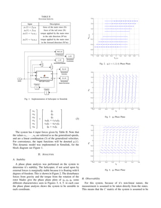
3. Fig. 5. q6 Phase Plane
TABLE III
SUMMARY OF PBH ANALYSIS
Eigenvalue Rank [λI − A|B]
0(×10) 8
±16.1j 12
diagonal (4). Because of this, the system is fully observable.
C = I12×12 (4)
However, in a real system the generalized speeds would not
be an easy measurement, a practical system would need a non-
linear estimator for these states. This could be implemented
using an Extended Kalman Filter [6]. Seeing as this is outside
the scope of the course, it’s implementation will be omitted
and the control design will be focused on.
C. Controllability
Because the system has 6 degrees of freedom and it only
has 4 inputs, it is intuitive that the system will have 2 un-
controllable positions. This is confirmed by linearizing about
the point x = 0 and applying a PBH analysis which yields
rank 8 for all but 2 states, which are fully controllable (Table
II-C). Also, the Kalman decomposition can be applied to find
exactly which subspace of the system states are uncontrollable
[4]. In the upright case, the forward direction is uncontrollable
(the helicopter must tilt to go forward) and a combination
of sideways movement and yaw is also uncontrollable. The
PBH and Kalman analysis supplied in Appendix A Shows
this clearly.
III. DESIGN
A. Methodology
Because of the uncontrollable characteristics of the system,
the control design methodology used to successfully imple-
ment the most important aspects of control was input-output
feedback linearization [2], [5]. First, because of the limitations
in control discussed in Section II-C, four states were picked
for control that were most important. In this particular system,
the altitude (q3) and rotations (q4, q5, q6) are best for a safety
control as the ground position of the helicopter can be allowed
to wander somewhat safely. With this decision made the
procedure for finding the control equations can be described.
First, the values of ˙qi are differentiated directly to get
the generalized accelerations. This is done so that the direct
derivative of the output is obtained rather than the derivative
of the more confusing generalized speeds. Once that is done
the derivatives of the generalized speeds are plugged in where
appropriate yielding.








w1
w2
w3
w4
w5
w6








=
∂
∂t








˙q1
˙q2
˙q3
˙q4
˙q5
˙q6








=









h1(q, ˙q, u, p)
h2(q, ˙q, u, p)
h3(q, ˙q, u, p)
h4(q, ˙q, u, p)
h5(q, ˙q, u, p)
h6(q, ˙q, u, p)









(5)
Using a CAS such as Mathematica [8], we can then solve
for the input forces p(t) as a function of w(t). So the that the
(easily designed) control input for the linear system (6) can
be translated back into input for the non-linear system (1).












q3
q4
q5
q6
˙q3
˙q4
˙q5
˙q6












=












0 0 0 0 1 0 0 0
0 0 0 0 0 1 0 0
0 0 0 0 0 0 1 0
0 0 0 0 0 0 0 1
0 0 0 0 0 0 0 0
0 0 0 0 0 0 0 0
0 0 0 0 0 0 0 0
0 0 0 0 0 0 0 0












+












0 0 0 0
0 0 0 0
0 0 0 0
0 0 0 0
1 0 0 0
0 1 0 0
0 0 1 0
0 0 0 1
















w3
w4
w5
w6



 (6)
The Mathematica output giving the control equations is
given in Appendix B
B. Controller
Once the control equations are calculated the controller is
implemented in Simulink [7]. The simple block diagram for
the system is shown in Figure 8.
IV. RESULTS
Using a height offset of 10 meters and randomly selected
initial angle values between -1.5 and 1.5 radians. The system
was tested first with (linear system) poles (7), then they were
doubled and the simulation was run again. The results are
shown in Figures 6 and 7 respectively.

4. Fig. 6. Slower Controller
Fig. 7. Faster Controller
Note that the faster controller results in the main rotor
actually driving downward. This tells us that the control
force is unreasonable in the second case. However, the first
controller has a reasonable settling time combined with a
reasonable actuation signal, and therefore it is the best choice
The poles selected for the final controller are therefore also

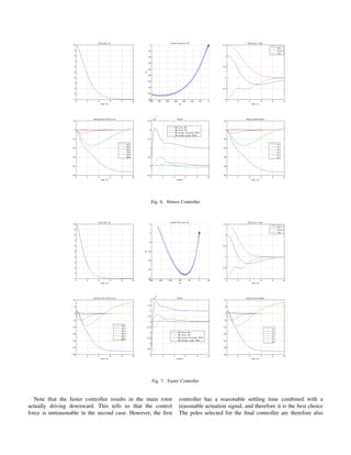
5. Fig. 8. Helicopter/Controller Simulink Model
given in (7).
−0.14 −1.6 −1.8 −2.0 −0.26 −2.8 −3.0 −3.2
(7)
V. CONCLUSION
In this paper a viable control design was developed and
testing in the Simulink simulation environment for and emer-
gency stabilization control on a two rotor helicopter. It shows
an approach to control design that can be used in very complex
non-linear systems. This will become more and more impor-
tant as flight done less by humans and more by autonomous
systems. As well, the safety benefits of this type of control
could save many lives.
Future developments for this controller could include a
way to control the second two states ”by-proxy” because the
controllability of the system changes as the states develop
in time. Obviously, a helicopter is ”fully controllable” in the
sense that a skilled pilot can fly and land it nearly anywhere,
so a more advanced controller based on this design might lead
to a two rotor helicopter that is fully autonomous.
REFERENCES
[1] L. Sandino, M. Bejar, A. Ollero, Tutorial for the application of Kane’s
Method to model a small-size helicopter. Proc. of the 1st Workshop
on research, development and education on Unmanned Aerial Systems
(RED-UAS 2011). Seville, Spain, Nov 30th - Dec 1st, 2011.
[2] K. Johnson, Course Notes: EENG517 Advanced Control Design, Col-
orado School of Mines, Spring Semester, 2015
[3] T. Kane, D. Levinson, Dynamics: Theory and Applications. The Internet-
First University Press. 2005.
[4] W. Brogan, Modern Control Theory, Third Edition, Prentice Hall, 1991
[5] J. E. Slotine, W. Li Applied Nonlinear Control Prentice Hall, 1991
[6] R. Brown, P. Hwang, Introduction to Random Signals and Applied
Kalman Filtering, Fourth Edition, Wiley, 2012
[7] MATLAB, Simulink and the Contols Toolbox Release 2014a, The Math-
Works, Inc., Natick, Massachusetts, United States.
[8] Wolfram Research, Inc., Mathematica, Version 10.1, Champaign, IL
(2015).

6. APPENDIX A
MATLAB CODE
A. test
APPENDIX B
INPUT-OUTPUT TRANSLATION EQUATIONS