Unmanned Airplane Autopilot Tuning

Petar Getsov et al Int. Journal of Engineering Research and Applications www.ijera.com
ISSN : 2248-9622, Vol. 4, Issue 7( Version 5), July 2014, pp.01-07
www.ijera.com 1 | P a g e
Unmanned Airplane Autopilot Tuning
Petar Getsov, Dimitar Yordanov, Svetoslav Zabunov
Abstract
This article considers different approaches for autopilot controller gain values adjustment. The correct autopilot
performance is tested using modeling methods. A variant of land-based autopilot is considered. Examined are
scenarios of UAV airplanes in level flight. The latter are applicable to tasks such as remote sensing, controlled
area surveillance, etc.
KEYWORDS: flight control, autopilot, safety.
I. INTRODUCTION
The main mode of unmanned airplane operation is the horizontal flight at a given altitude aiming at earth
surface surveillance of certain objects and areas. Another purpose of using UAV airplanes in level flight is to
fulfill remote sensing applications dealing with study of phenomena, geophysical activities, etc. Such a flight is
usually an autonomous one and is controlled by an onboard computer. Also such flight is usually taking place in
the zone beyond direct line-of-sight. The autopilot sustains predefined flight route in the presence of
disturbances. For the qualities of mission being executed one can measure flight trajectory in the ground control
station. Direct line-of-sight flight may be conducted even without an onboard computer, but instead using a
land-based computer connected to the ground control station. The land-based computer implements an autopilot
that controls the flight over a predefined route. This variant is preferred in the discussed setup used for modeling
of the direct line-of-sight flight. The utilized airplane possesses the following aerodynamic and
mass/dimensional data:
Mass = 50 kg;
Cy =4.72, Cz=-0.31, Czδn=-0.14, mz
Cy =-0.13 , mx
 =-0.058, my
 =-0.12,
mz
z =-8.99, mx
x=-0.33, my
y=-0.1 , mx
y=-0.11 , my
x=0.11, mz

=-4.3,
mz
v=-1.09, mx
e=-0.24 , my
n =-0.07 , mx
n=-0.01,
Sroll= 2.14 m2; lroll =5.06 m; broll=0.42 m; Ix=21.4 kg.m2; Iy=29.3 kg.m2; Iz
= 12.4 kg.m2
Flight altitude is from 10 m to 500 m, speed – 100 km/h.
II. Autopilot for turning maneuver
The most suitable autopilot model for the horizontal plane trajectory control is the roll control, according to
which the turns are carried out using the ailerons and performing banking maneuvers. The aileron deflection law
can be described as follows:
e e set е set е x
 K   K   dt K x    (  )   (  )  1
( ) ( ) set e programmed programmed set _by _ pilot Z programmed   K     K Z Z 
1
( ) _ _ _ 
 
Тp
k
K set by pilot pilot pilot program   
From the above formulae it is obvious that an astatic autopilot controller is discussed. The integral element
of the controller holds the roll angle traced by the autopilot program, while the pilot on the ground may, in a
combined mode of control, perform momentary and short-timed adjustments to the roll angle. The combined
mode of control allows the pilot on the ground to introduce corrections by holding the joystick (manipulator) in
the ground control station at an inclined angle until the desired corrections have been reached. The discussed
modeled flight scheme includes manual takeoff and altitude climb up to 100 m with right turn. After this point
the autopilot engages and controls the aircraft along a circular route and then performs landing. The autopilot
tuning routine consists of controller gain values selection and following verification of their correctness using
RESEARCH ARTICLE OPEN ACCESS

modeling of transient processes and modeling of the whole flight. The theory [1] gives tentative formulae for
choosing the controller gains e e e e z K , K K x , K , K 1 ,
  
.
The gain figures

e K , x
e K
and 1e, K are defined by time treg of the roll transient process and an
admissible small overshoot. The results of the theoretical calculations of the gain values are verified using
modeling methods. Systems that include an integral part apply for the law with speed feedback [1 – p.382-383].
This law may be transformed as follows:
( ) 2
e e e e set p  p   p  i  
( )
1
e e e e set р
  p     i  
These laws are transformed into a more popular form of the gain figures:
x
e e K   ;
  e e  K ; e e i K1 
The roll transient process regulation time is chosen at treg=5s.
If the controlled airplane‟s mass/dimensional and aerodynamic values are known the gain figures may be
calculated

e K , x
e K
and 1e, K using the following formulae:
53.55
2
1.125 28 2.14 5.06
21.4
0.24
2
2 2
3 
  


    
V Sl
I
m
b
x
x
v  
(1/s2)
The integral element gain has the measure of (1/s):
0.18
53.55 5
1218 1218
3 3
3
1 

 
reg
e b t
K
The proportional element gain has no measure:
0.34
2.67
0.18 5
2.67
1 

  e reg
e
K t
K
6.65
4
1.125 28 2.14 5.06
21.4
0.33
4
2 2
1 
  


    
VSl
I
m
b
x
x
x  
(1/s)
0.035
53.55 5
42.7 42.7 6.65 5
3
1 

 



reg
reg
e b t
b t
Kx
(s)
If the calculated value for x
e K
is negative that means the aircraft in this mode has good damping and we may
set x  0
e K
. Then only a rudder dumping will be enough for stabilizing the airplane‟s yaw motion. The yaw
damping will affect both channels, because, due to the interconnection between yaw and roll rotations, damping
the yaw motion will damp the roll motion too.
The yaw gain is [1 – p. 130]:
3
2 1 4 (0.4 0.8) ( )
a
a a a
K y
y
  
 
, where
y
y
I
m V S
a
y
2
2
1
  
  ,
y
y
I
m V S
a
2
2
2
  
  ,

y
y
I
m V S
a
y
2
2
3
  
 
m
c V S
a z
2 4
 
 
After substitution with the characteristic quantities for the studies aircraft (taking into account that
V
y
y 2
 
  ),
it follows:
 0.0080.16 y
y K
(s)
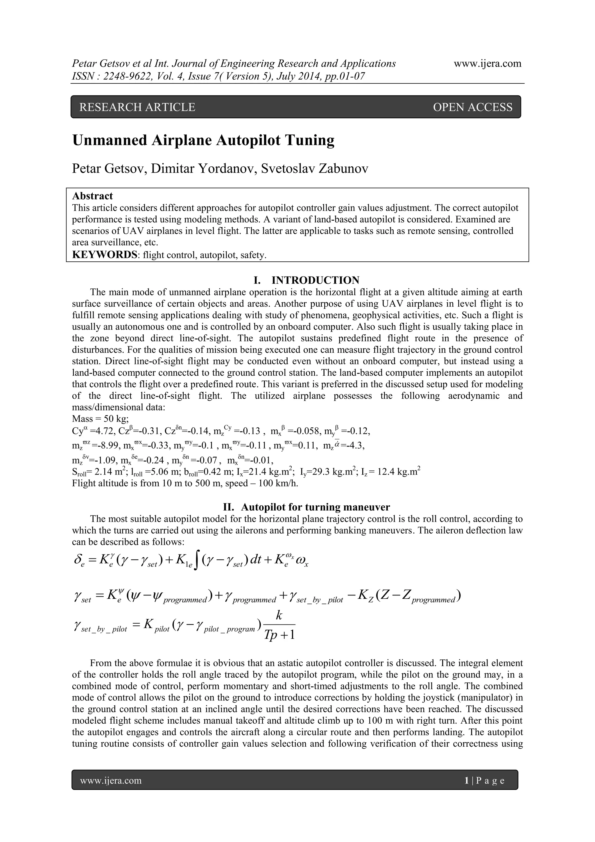
Fig.1. „Simulink‟ results of the transient process after setting a desired roll angle in the astatic autopilot
The gain figures

e K and
Z
e K for the simplest control law are derived using equations from the theory [1 –
p.397], while the course settling time for a small unmanned airplane may be chosen at tstl =25...35s. Pitch
control over horizontal maneuvers with speed of 28 m/s (100 km/h) is about
0  6 10 avg  .


cos
9.48
stl
e gt
V
K 
For t=25…35s it is accepted 1 0.78
9.81 0.985 (25 35)
9.48 28
 
  

 
e K
0.11 0.2
9.81 0.985 (25 35)
22.468 57.3
cos
22.468 57.3
2 2  
  




 reg
Z
e gt
K (deg/m)

The command ( ) set Z programmed   К Z  Z is switched on only under boundary conditions of the Z
coordinate, defined by the model. Approaching landing this command is engaged when Z<400m. This
command is defined in the flight program in the ground control station.
Using modeling approach, the transient process is verified, i.e. the deflections of the ailerons and rudder in
the presence of typical signal (step-shaped roll angle signal setting). Fig.1 presents the results of the transient
process modeling of the lateral motion with mutually conditioned roll and slipping angular motions.
Overshoot of the desired roll angle in the beginning of the transient process (about t≈2,5s) is due to the
integral part. When modeling isolated roll motion using integral part in the controller a monotonous process is
obtained with gradual approach to the desired value without overshoot, but the static error during constant roll
disturbances.
III. Autopilot for control and stabilization of the flight altitude
Automatic control and stabilization of the major coordinate is the deviation of the airplane mass center
along the vertical axis. This deviation in the real aviation is measured by a barometric altimeter, radio-altimeter
or an inertial system. In the modeling process the altitude is obtained by integrating of the differential equations.
The longitudinal control channel (pitch control PΔН achieved using the elevator) is maintained satisfactorily
by the autopilot under most practical disturbances even when implemented using the simplest law:
( ) ( ) set
Н
v v set v z v   K    K z  K Н Н  
Under constant disturbances the statistical errors depend on the magnitude of the major coordinate gain
H
e K . The theory [1 – p.292] gives the following optimal gain figure for subsonic unmanned airplanes. This
figure is appropriate for smooth rate of climb and altitude stabilization of such airplanes:
 0,18 H
e opt K (deg/m)
During modeling, the elevator autopilot adjustment requires at least three gains to be estimated in the
control law:
Н
v v v K , K z , K  
The theory presents formulae [1 – p.135] to calculate the gain z
v K
:
      2 K z a a
v
The calculations show that the latter equation has several cases:
1. Two roots, a negative and positive one. The positive root is used z  0
v К
;
2. Two negative roots – a very good self-damping of the airplane ( need airplane   ) or a small reserve of
balance along the longitudinal axis (excessive aft center of gravity) or neutrality – we assume z  0
v К 
;
3. Two complex roots – instability under overload (such case with the unmanned aircraft is not considered).
Using the recommended algorithm we set the needed value of the relative damping of the oscillations about
the ОZ axis to   0.75 1 . Using the equation       2 K z a a
v two possible values are derived
(usually one positive and one negative value) and the positive value is chosen. In this equation
3
1 4 5 4 2
c
c c c c
a need    
 ;
2
3
1 4 2
2
1 4 5 ( ) 4 ( )
c
c c c c c c need    




Coefficients c1, с2 , c3, c4, c5, c6 are determined by the following table using the chosen aerodynamic and
mass/dimensional characteristics of the unmanned airplane [appendix 2 in 1 – p.432]:
Coefficient c1 [1/s] ≈ 4,3
z
a
z
z
I
m VSb c 1 2
2  
 
Coefficient c2 [1/s2] ≈19.6
z
z a
I
m V Sb c 2 2
2  

z
y a
Cy
z
I
m C V Sb
2
2  
 
Coefficient c3 [1/s2] ≈34
z
a
в
z
I
m V Sb c 3 2
2  

Coefficient c4 [1/s] ≈3.2
m
cy cx VS c 2
( )
4
  
 m
cy VS
2
 

Coefficient c5 [1/s] ≈2.06
z
z a
I
m VSb c 5 2
2  

Coefficient c6 [m/s.deg] ≈0.49
5 57.3
c  V
Coefficients a  0.09 ;  0.0345
0.116 2       K z a a
v s
The gain figure multiplied by the pitch angle signal is obtained according to formulae [1 – p.193..195]:
1
(0.9 1) 4 


c
v opt k
c
K
, where
2.8
1 4 2 3 4
3 4 
 

c c c K c c
c c
k
z
v
c 
Under modeling, the increase of this figure leads to oscillations in the middle of the process, while its
decrease prolongs the process duration. For the considered unmanned airplane according to modeling data, best
results are  0.751 
v opt K .
On the basis of the conducted calculations and modeling, the ensemble of gain figures of the autopilot APΔН
is:
 0.18 H
e opt K (deg/m);  0.751 
v opt K ; K z s
v  0.116 
.
IV. Modeling of flight “over a circle”
The flight over a circle is a typical maneuver during takeoff and landing tutoring. In the current case a
maneuver similar to a “flight in a circle” is modeled using manual takeoff with turn to the right, automatic
course change with two right turns of 1800 and climb up to 300 m, descent and landing in the direction of
takeoff with minimal deviation of the Z coordinate. The trajectory results are shown on Fig.2-5.

Fig.2. Horizontal projection of the trajectory Fig.3. Vertical projection of the trajectory
Fig.4. Decreasing of the lateral deviation ΔZ(m) before landing on the runway under side-wind from the left of the airplane with 2 m/s. The landing is programmed with correction to the course.
Fig.5. Change of flight altitude H(m) in the last seconds of automatic landing The modeled typical flight has the following gains for the autopilot:

 0.9 
e K ,  0.11 Z
e K deg/m, K x s
e  0.035 
, K s y
н  0.16 
,  0.34 
e K , 0.18 1  e K ,
 0.18 H
e opt K deg/m; , 1 
v opt K , K z s
v  0.11 
.
When the signal line from the ground control station to the airplane is interrupted it is advisory to have an
emergency mode of the autopilot. This may be for example restoration of the course and altitude of flight as it
was before signal drop.
For the correct work of the autopilot it is required during the modeling process that the angles of attack and
normal overloads to be verified while executing the flight program. The safe values should not be exceeded.
Generally, the presence of one inertial element with time constant of 2 s at the output of the flight program is
enough to fool proof the normal overloads and angles of attack (the autopilot works “softly”).
V. Conclusions
 The carried out flight modeling confirms the correct choice of gain figures for the autopilot.
 When the range of flight altitudes and speeds is narrow (as with the unmanned airplanes of the discussed
class – 50 kg), we may keep the gain figures constant during flight.
References
[1] Mihalev I.A., B.N. Okoemov, I.G. Pavlina, M.S. Chikulaev, N.M. Eidinov. Automatic airplane control
systems – methods for analysis and synthesis, ”Mashinostroenie” publ., Moscow 1971

Unmanned Airplane Autopilot Tuning

More Related Content

What's hot

Viewers also liked

Similar to Unmanned Airplane Autopilot Tuning

Recently uploaded

Unmanned Airplane Autopilot Tuning