The thesis by Albert Farré Gabernet addresses the modeling and control of an F-16 aircraft with bounded actuators as part of his Master's degree in Mechanical and Aerospace Engineering. It covers the development of nonlinear and linear models, Linear Parameter Varying (LPV) systems, and controller design, including various techniques for achieving altitude hold and signal tracking. The document concludes with simulations demonstrating the performance of the proposed control methods under different conditions.


![List of Figures
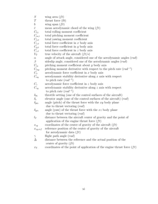
2.1 Definition of roll, yaw and pitch angles and main control surfaces in a
general aircraft . . . . . . . . . . . . . . . . . . . . . . . . . . . . . . 5
2.2 Definition of axes and aerodynamic angles (obtained from [13]) . . . . 6
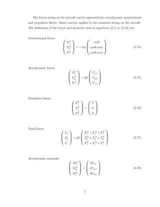
2.3 Scheme of the engine model used with the functions TGEAR, PDOT
and THRUST. Dashed circles show the inputs, plain circles show the
outputs. . . . . . . . . . . . . . . . . . . . . . . . . . . . . . . . . . . 9
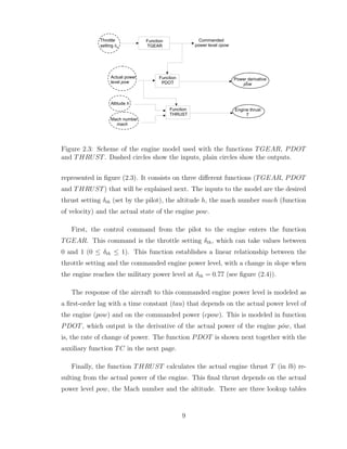
2.4 Relationship between the throttle setting and the engine power level.
Note the change in slope around δth = 0.77 . . . . . . . . . . . . . . . 11
2.5 Scheme of the thrust vectoring and its relevant angles . . . . . . . . . 12
2.6 Relevant angles and axes in the longitudinal model . . . . . . . . . . 24
2.7 Scheme of the longitudinal model of the aircraft with and without the
thrust vectoring . . . . . . . . . . . . . . . . . . . . . . . . . . . . . . 24
2.8 Nonlinear longitudinal model of the F − 16 aircraft implemented in
Simulink r
° . . . . . . . . . . . . . . . . . . . . . . . . . . . . . . . . . 25
2.9 Plots of the different aerodynamic coefficients . . . . . . . . . . . . . 26
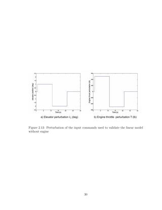
2.10 Perturbation of the input commands used to validate the linear model 27
2.11 Time responses for a perturbation in δe at V = 160ft/s and α = 35.01◦
28
2.12 Time responses for a perturbation in δth at V = 160ft/s and α = 35.01◦
29
2.13 Perturbation of the input commands used to validate the linear model
without engine . . . . . . . . . . . . . . . . . . . . . . . . . . . . . . 30
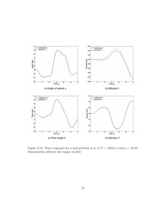
2.14 Time responses for a perturbation in δe at V = 160ft/s and α = 35.01◦
(linearization without the engine model) . . . . . . . . . . . . . . . . 31
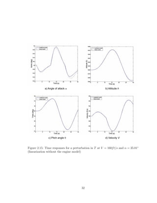
2.15 Time responses for a perturbation in T at V = 160ft/s and α = 35.01◦
(linearization without the engine model) . . . . . . . . . . . . . . . . 32
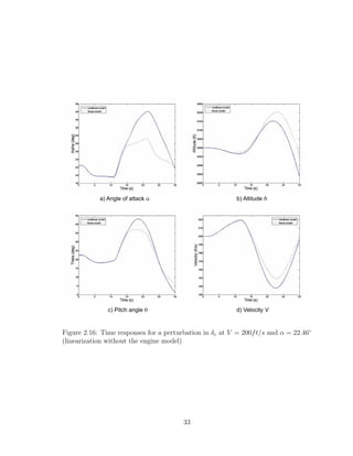
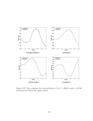
2.16 Time responses for a perturbation in δe at V = 200ft/s and α = 22.46◦
(linearization without the engine model) . . . . . . . . . . . . . . . . 33
2.17 Time responses for a perturbation in T at V = 200ft/s and α = 22.46◦
(linearization without the engine model) . . . . . . . . . . . . . . . . 34
vi](https://image.slidesharecdn.com/msthesisafarre07-240828145330-68543729/85/MSthesis-control-for-system-s-with-bounded-actuators-pdf-7-320.jpg)
![3.1 Scheme of the LPV model . . . . . . . . . . . . . . . . . . . . . . . . 38
3.2 Time responses for a perturbation in δe at V = 180ft/s and α = 33.5◦
(linear system obtained using an LPV model) . . . . . . . . . . . . . 42
3.3 Time responses for a perturbation in δe at V = 180ft/s and α = 33.5◦
(linear system obtained using an LPV model) . . . . . . . . . . . . . 43
3.4 Extended scheme of the LPV model, in which the LPV region consists
on different squares with coincident sides . . . . . . . . . . . . . . . . 44
4.1 Plot of the saturation effect . . . . . . . . . . . . . . . . . . . . . . . 46
4.2 Scheme of a plant with an open loop controller and a representation of
the actuator. The actuator is represented by a saturation block and a
delay transfer function . . . . . . . . . . . . . . . . . . . . . . . . . . 47
4.3 Estimate for the smallest invariant set associated with ωmax without
actuator limits (large ellipsoid) and ωnom (small ellipsoid) for Knom.
Parallel lines show region where Knom is not saturated (figure obtained
from [17]) . . . . . . . . . . . . . . . . . . . . . . . . . . . . . . . . . 56
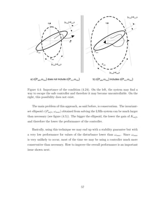
4.4 Importance of the condition (4.24). On the left, the system may find a
way to escape the safe controller and therefore it may become uncon-
trollable. On the right, this possibility does not exist. . . . . . . . . . 57
4.5 Invariant set associated with ωmax and Ksafe compared to linear case
(figure obtained from [17]) . . . . . . . . . . . . . . . . . . . . . . . . 58
5.1 Scheme of the elevator actuator . . . . . . . . . . . . . . . . . . . . . 66
5.2 Bode plot of the elevator actuator . . . . . . . . . . . . . . . . . . . . 68
5.3 Probability of exceedance of turbulence intensity as a function of altitude 70
5.4 Effect of expanding the saturation limits, showing how Pnom,max in-
cludes Pnom,min (ulim,min ≤ ulim,max) . . . . . . . . . . . . . . . . . . . 75
5.5 Plot of the wind velocity obtained from a moderate disturbance and
the open loop response (altitude) of the linear model of the aircraft to
this disturbance . . . . . . . . . . . . . . . . . . . . . . . . . . . . . . 80
5.6 Plot of the wind velocity obtained from a moderate disturbance and
the closed loop response (altitude) of the linear model of the aircraft
to this disturbance . . . . . . . . . . . . . . . . . . . . . . . . . . . . 92
vii](https://image.slidesharecdn.com/msthesisafarre07-240828145330-68543729/85/MSthesis-control-for-system-s-with-bounded-actuators-pdf-8-320.jpg)
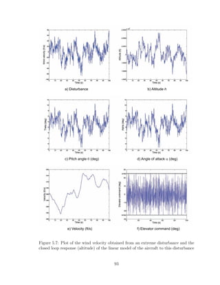
![5.7 Plot of the wind velocity obtained from an extreme disturbance and
the closed loop response (altitude) of the linear model of the aircraft
to this disturbance . . . . . . . . . . . . . . . . . . . . . . . . . . . . 93
5.8 Effect of the transfer function in (5.27) to the commanded flight path
angle γcmd (the amplitude of γcmd may vary depending on the case of
study) . . . . . . . . . . . . . . . . . . . . . . . . . . . . . . . . . . . 94
5.9 Nonlinear ±1.5◦
doublet response (stable case) with Knom . . . . . . 95
5.10 Nonlinear ±3◦
doublet response (stable case) with Knom . . . . . . . 96
5.11 Nonlinear ±3◦
doublet response (stable case) with Knom and Ksafe . . 97
5.12 Nonlinear ±3◦
doublet response (stable case) with Knom, K1, K2 and
Ksafe . . . . . . . . . . . . . . . . . . . . . . . . . . . . . . . . . . . . 98
5.13 Nonlinear ±5◦
doublet response (stable case) with Knom, K1, K2 and
Ksafe . . . . . . . . . . . . . . . . . . . . . . . . . . . . . . . . . . . . 99
5.14 For comparison purposes: nonlinear ±1◦
doublet response (stable case)
with an LTI nominal controller (extracted from [13]) . . . . . . . . . 100
5.15 For comparison purposes: nonlinear ±2◦
doublet response (stable case)
with/without an LTI antiwindup compensator (extracted from [13]) . 101
5.16 Nonlinear ±1.5◦
doublet response (unstable case) with Knom . . . . . 102
5.17 Nonlinear ±3◦
doublet response (unstable case) with Knom . . . . . . 103
5.18 Nonlinear ±3◦
doublet response (unstable case) with Knom and Ksafe 104
5.19 Nonlinear ±3◦
doublet response (unstable case) with Knom, K1, K2
and Ksafe . . . . . . . . . . . . . . . . . . . . . . . . . . . . . . . . . 105
5.20 Nonlinear ±3.5◦
doublet response (unstable case) with Knom, K1, K2
and Ksafe . . . . . . . . . . . . . . . . . . . . . . . . . . . . . . . . . 106
viii](https://image.slidesharecdn.com/msthesisafarre07-240828145330-68543729/85/MSthesis-control-for-system-s-with-bounded-actuators-pdf-9-320.jpg)
![Abstract of the Thesis
Controllers for Systems with Bounded Actuators:
Modeling and control of an F-16 aircraft
by
Albert Farré Gabernet
Master of Science in Mechanical and Aerospace Engineering
University of California, Irvine, 2007
Professor Faryar Jabbari, Chair
Actuator capacity limitation has been a major topic of control research in recent
decades and plays a major role in the flight control system design area, specially
in the high angle of attack region. The development of linear matrix inequalities
(LMIs) and other optimization techniques provided a new framework that facilitates
the design of controllers dealing with saturation, making it easier to obtain stability
and performance guarantees for the designed controllers. These saturation techniques
can be classified into two groups: anti-windup and direct approach. Recently, a new
method combining both groups has been proposed in [17] for the disturbance atten-
uation problem, although it can be easily extended to include the tracking problem.
This thesis will show the potential of this new combined technique applied to com-
mon aircraft problems (altitude hold and tracking a reference command) in which
saturation problems have been reported.
xiii](https://image.slidesharecdn.com/msthesisafarre07-240828145330-68543729/85/MSthesis-control-for-system-s-with-bounded-actuators-pdf-14-320.jpg)
![the development of linear matrix inequalities (LMIs) and other optimization tech-
niques have provided a framework in which the stability and performance guarantees
are more rigorous than in the past.
The techniques used to deal with saturation can be classified into two groups. The
first group uses the so-called anti-windup scheme, which consists on an augmentation
on top of a nominal controller that was designed without taking saturation into ac-
count. Once the nominal controller saturates, the anti-windup scheme tries to modify
the value of the control signal such that the closed loop system behaves well. It is
the most extended approach to avoid saturation problems in control design, specially
in cases in which saturation is not likely to occur because the nominal controller is
used most of the time. The second group can be called the direct approach method,
in which saturation of the controller is taken into account from the beginning of the
design process. In this approach, controllers are designed in order to avoid saturation
even for the worst-case scenario (e.g. worst case disturbance). Since this worst case
may not occur, it is usually a conservative method.
Recently, a new method combining both design schemes has been proposed in [17]
for the disturbance attenuation problem. The main advantage of this method is that
it can be applied to unstable systems and that it can be extended, in a straightforward
fashion, to include some level of controller scheduling in order to reduce conservatism.
Therefore, the objective of this thesis is to demonstrate the potential of this new
method applied to flight control system design. Two main maneuvers are simulated
with the objective to saturate the control surfaces and check the performance of this
new technique: altitude hold (disturbance attenuation problem) and flight path angle
tracking (model following problem).
This thesis is organized as follows.
In chapter 2 a longitudinal nonlinear model of an F −16 aircraft is developed and
implemented using Matlab r
° and Simulink r
°. The equations used and the assump-
tions considered are shown, as well as the linearization and validation processes.
2](https://image.slidesharecdn.com/msthesisafarre07-240828145330-68543729/85/MSthesis-control-for-system-s-with-bounded-actuators-pdf-16-320.jpg)

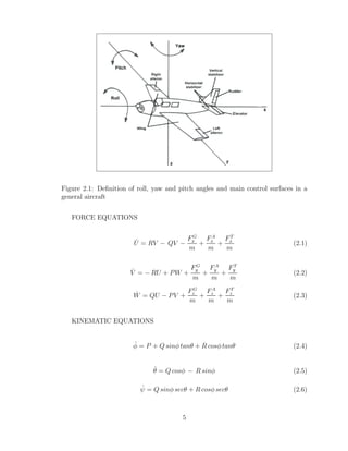
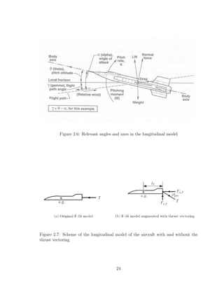
![Chapter 2
Modeling of an F-16 aircraft
Modeling is one of the most important parts in control engineering. It allows to
mathematically represent the desired system and simulate it via appropriate simula-
tion programs. This way, computer simulations can be run and the controllers can
be tested.
In this section, a nonlinear model of an F-16 aircraft will be studied. First, a
general 6 degree-of-freedom (DOF) model is shown and then reduced to a decoupled
longitudinal 3 DOF model.
2.1 Nonlinear 6 degree-of-freedom aircraft model
According to [18] and [13], the equations of motion of an aircraft in the body-fixed
reference axes can be expressed as:
4](https://image.slidesharecdn.com/msthesisafarre07-240828145330-68543729/85/MSthesis-control-for-system-s-with-bounded-actuators-pdf-18-320.jpg)
![Figure 2.2: Definition of axes and aerodynamic angles (obtained from [13])
MOMENT EQUATIONS
ΓṖ = Jxz(Jx − Jy + Jz)PQ − [Jz(Jz − Jy) + J2
xz]QR + JzMx + JxzMz (2.7)
JyQ̇ = (Jz − Jx)PR − Jxz(P2
− R2
) + My (2.8)
ΓṘ = [(Jx − Jy)Jx + J2
xz]PQ − Jxz(Jx − Jy + Jz)QR + JxzMx + JxMz (2.9)
Γ = JxJz − J2
xz (2.10)
NAVIGATION EQUATIONS
ṗN = Ucθcψ + V (sφsθcψ − cφsψ) + W(sφsψ + cφsθcψ) (2.11)
ṗE = Ucθcψ + V (cφcψ + sφsθsψ) + W(cφsθsψ − sφcψ) (2.12)
ḣ = Usθ − V sφcθ − Wcφcθ (2.13)
6](https://image.slidesharecdn.com/msthesisafarre07-240828145330-68543729/85/MSthesis-control-for-system-s-with-bounded-actuators-pdf-20-320.jpg)
![For purposes of linearizing the equations of motion and studying the dynamic
behavior, it is recommended to have the velocity equations expressed in wind or
stability axes variables, which are the true airspeed and the aerodynamic angles of
the aircraft axes with respect to the wind axes (VT , α and β) (2.19)-(2.21). The
stability reference frame is an special frame fixed in the body that is used in the
study of small deviations from a nominal flight condition. It differs from the body
frame shown in (2.2) because the x-axis is chosen as the projection of the aircraft
true velocity into the plane defined by the body axes XZ (the y-axis of this stability
frame coincides with the body y-axis). The wind frame has its x-axis in the direction
of the aircraft’s true velocity and the z-axis is the same as the body z-axis.
VT =
√
U2 + V 2 + W2 (2.19)
α = tan−1
³W
U
´
(2.20)
β = sin−1
³ V
VT
´
(2.21)
Using the definitions (2.19) to (2.21), we can rewrite the force equations (2.1) to
(2.3) with the new states:
˙
VT =
1
m
(Fxcα cβ + Fysβ + Fzcβ sα) (2.22)
β̇ =
1
mVT
(−Fxcα sβ + Fycβ − Fzsα sβ) + P sα − R cα (2.23)
α̇ =
1
mVT
³
− Fx
sα
cβ
+ Fz
cα
cβ
´
− P cα tanβ + Q − R sα tanβ (2.24)
2.1.1 Engine model
The engine of an F-16 aircraft is an afterburning turbofan engine. A model of this
engine is included in [12] and can be also found in [18]. A scheme of this model is
8](https://image.slidesharecdn.com/msthesisafarre07-240828145330-68543729/85/MSthesis-control-for-system-s-with-bounded-actuators-pdf-22-320.jpg)
![containing this data, depending on the power level at which the engine is working:
idle, military or maximum. These tables can be found in [18].
Since the final thrust depends on the actual power level, the actual power level
has to be included in the state vector of the system. This state is called pow, is
dimensionless and ranges from 0 to 100. The variations in time of pow depend on the
thrust setting δth set by the pilot and the algorithm in function PDOT.
FUNCTION PDOT ( cpow , pow )
if (cpow ≥ 50.0) then
if (pow ≥ 50.0) then
tau = 5.0
paux = cpow
else
paux = 60.0
tau = tc(paux − pow)
end
else
if (pow ≥ 50.0) then
tau = 5.0
paux = 40.0
else
paux = cpow
tau = tc(paux − pow)
end
end
10](https://image.slidesharecdn.com/msthesisafarre07-240828145330-68543729/85/MSthesis-control-for-system-s-with-bounded-actuators-pdf-24-320.jpg)
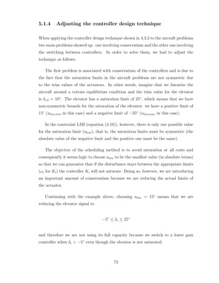
![Figure 2.5: Scheme of the thrust vectoring and its relevant angles
Thrust vectoring model
In the high angle of attack region, the usual control surfaces of the aircraft may not
be sufficient to control the aircraft and obtain the desired performance. Vectoring
the thrust is one option to extend the capabilities of the aircraft in this region.
Usually, the thrust of the engine is directed through the body x-axis. Therefore,
the propulsive force of the engine has only one component in this axis, having no
effect on the other axes (check equation (2.16)). By vectoring the thrust, we are able
to direct this propulsive thrust into any direction. The main benefit is that now the
propulsive force of the engine has components in all the body axes, obtaining a better
performance of the engine for the same amount of thrust.
Considering a deflection of the thrust vector in the pitch (δptv) and yaw (δytv)
planes as in figure (2.5), the new propulsive forces can be written as (2.25)(according
to [13]). These new components of the propulsive forces also produce moments along
the yaw and pitch axes, with a moment arm of lT = xcg − xT (2.26).
12](https://image.slidesharecdn.com/msthesisafarre07-240828145330-68543729/85/MSthesis-control-for-system-s-with-bounded-actuators-pdf-26-320.jpg)
![Propulsive forces with thrust vectoring become
FT
x
FT
y
FT
z
= T
cosδptv sinδytv
sinδytv
−sinδptv cosδytv
(2.25)
Propulsive moments due to thrust vectoring become
MT
x
MT
y
MT
z
=
0
lT FT
z
lT FT
y
(2.26)
2.2 Longitudinal model
In this section we will present the actual model that we implemented for the simula-
tions. It is based on the fact that, under certain conditions, the equations of motion
can be decoupled a longitudinal mode (motion in the vertical plane) and into a lateral
mode (motion in the horizontal plane). These conditions are:
• The aircraft is on a wings-level steady-state flight condition (implies φ = 0).
• The sideslip angle is very small ( β ≃ 0 ).
• the roll and yaw rates (P and R) are small.
Assuming these assumptions hold and including the thrust vectoring system seen
before (δytv = 0 due to the longitudinal assumptions), the state variables are
x = [ VT α q θ pow h ]T
13](https://image.slidesharecdn.com/msthesisafarre07-240828145330-68543729/85/MSthesis-control-for-system-s-with-bounded-actuators-pdf-27-320.jpg)
![and the equations of motion can be rewritten as follows:
˙
VT =
q̄Sc̄
2mVT
[Cxq(α)cos(α) + Czq(α)sin(α)]q − gsin(θ − α) +
+
q̄S
m
(Cx(α, δe)cos(α) + Cz(α, δe)sin(α)) +
T
m
cos(α + δptv) (2.27)
α̇ = [1 +
q̄Sc̄
2mV 2
T
(Czq(α)cos(α) − Cxq(α)sin(α))]q +
g
VT
cos(θ − α) +
+
q̄S
mVT
(Cz(α, δe)cos(α) − Cx(α, δe)sin(α)) −
−
T
mVT
sin(α + δptv) (2.28)
q̇ =
q̄Sc̄
2JyVT
[c̄Cmq(α) + ∆Czq(α)]q +
+
q̄Sc̄
Jy
[Cm(α, δe) +
∆
c̄
Cz(α, δe)] −
lT T
Jy
sin(δptv) (2.29)
θ̇ = q (2.30)
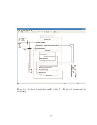
ḣ = VT cosα sinθ − VT sinα cosθ (2.31)
The time derivative of the state pow has been presented in section 2.1.1, where the
function PDOT calculates the time derivative of pow as a function of itself and the
commanded power level set by the pilot. Information about the engine can obtained
from a more detailed model of the engine, available in [12]. Figure (2.8) shows the
implemented F − 16 aircraft model in Simulink r
°.
2.2.1 Aircraft description
The parameters used to implement the model of the F-16 aircraft are shown in table
(2.1).
The aircraft longitudinal model uses three different actuators. The first one cor-
responds to the elevator angle δe, which mainly affects the value of the aerodynamic
coefficients. The second one is the thrust setting δth, that affects the value of the
motor thrust T. The third one, δptv is the vectoring angle of the thrust. Table (2.2)
14](https://image.slidesharecdn.com/msthesisafarre07-240828145330-68543729/85/MSthesis-control-for-system-s-with-bounded-actuators-pdf-28-320.jpg)
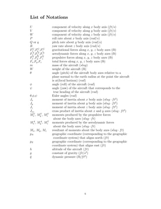
![Table 2.1: Mass and geometric properties of the aircraft
Parameter Value
Weight W (lb) 20500
Wing area S (ft2
) 300
Mean aerodynamic chord c̄ (ft) 11.32
Reference cg location xcg,ref (ft) 0.35c̄
Moment of inertia Jy (slug ft2
) 55814
Table 2.2: Models of the control actuators
Actuators Position limit Rate limit Time constant
Elevator δe ±25◦
60◦
/s 0.0495s
Thrust vectoring δptv ±17◦
60◦
/s 0.07s
shows the relevant parameters of these actuators. The response of the elevator and
the thrust vectoring actuators is modeled in both cases as first-order systems.
In this master’s thesis, the delay in the response of the elevator (with a time
constant of 0.0495 s) is considered in the simulations and the design of the con-
trollers. However, the thrust vectoring actuator will not be considered, although it is
introduced in the model for further simulations and investigations.
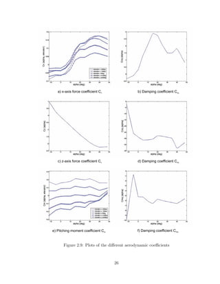
2.2.2 Aerodynamic data
The aerodynamic data used in this thesis was obtained in a series of wind tunnel tests
on a subscale model of an F-16 airplane ([12]). This data consists on 50 look-up tables
and covers a wide range of angle of attack and of sideslip angle (−20◦ ≤ α ≤ 90◦
and
−30◦ ≤ β ≤ 30◦
). However the actual techniques for modeling in the poststall region
are not accurate, so the reduced data presented in [18] is used.
This reduced data (10 look-up tables) covers a range for the angle of attack be-
tween −10 and 45 degrees and the dependence on β has been approximated in some
cases. The number of look-up tables is finally reduced to 4 by considering only the
15](https://image.slidesharecdn.com/msthesisafarre07-240828145330-68543729/85/MSthesis-control-for-system-s-with-bounded-actuators-pdf-29-320.jpg)
![A =
−0.1656 −10.7137 −7.2815 −32.1740 0 3.951e − 4
−0.0018 −0.0981 0.9276 0 0 4.2663e − 6
0 −0.6252 −0.4673 0 0 0
0 0 1.0000 0 0 0
0 0 0 0 −1.0000 0
0 −160.0000 0 160.0000 0 0
(2.44)
B2 =
−4.0478 −9.2839 0
−0.0253 −0.0828 0
−0.8992 −1.8471 0
0 0 0
0 0 64.9400
0 0 0
(2.45)
From the B matrix we can see that the thrust setting δth (3rd column) only affects
the pow state (4th row). Then, by checking the A matrix, it can be seen that the pow
state (4th column and row) only affects itself, having no effect on the other states.
Therefore, a change in the thrust setting produces a change in the pow state, but this
change does not translate into changes in the other states. The pow state is decoupled
and this is the reason why the linear model does not follow the nonlinear model for
changes in δth.
In order to avoid this problem, the engine model has to be removed from the
general nonlinear aircraft model. Then, the control input δth disappears and is sub-
stituted by T (engine thrust). This means that our control signal is directly the
output of the engine. Table (2.3) shows the physical limitations of the engine thrust
T [18], that will be used in the simulations chapters to determine whether the thrust
actuator is saturated or not. We will not consider any delay effects in the thrust,
since we interpret that they depend on the engine model.
20](https://image.slidesharecdn.com/msthesisafarre07-240828145330-68543729/85/MSthesis-control-for-system-s-with-bounded-actuators-pdf-34-320.jpg)
![Chapter 3
Linear Parameter Varying (LPV)
systems
One of the main problems in modeling real life systems is the presence of uncer-
tainties because it affects the validity of the model. Out of the two main families of
linear systems uncertainties (dynamical input-output and state space uncertainties,
[1]), state space uncertainties are particularly interesting.
State space uncertainties arise due to the fact that the physical parameters on
which the system depends may vary with time, and they directly affect the state
space matrices. The wider the operating envelope of the system, the more the pa-
rameter (and consequently the system matrices) change. This often makes the system
nonlinear, since the variation depends on the value of the states.
An example of state space uncertainty would be the weight of an aircraft. During
flight, fuel is burned and the weight of the airplane is reduced, changing the state
space matrices.
35](https://image.slidesharecdn.com/msthesisafarre07-240828145330-68543729/85/MSthesis-control-for-system-s-with-bounded-actuators-pdf-49-320.jpg)
![where A ǫ ℜ nxn
, B ǫ ℜ mxn
and ρ(t) is a time-varying parameter vector (scheduling
vector) not known in advanced although it can be measured in real time and it
moves inside a certain bounded region P known a priori. If the scheduling vector
ρ(t) includes some of the states of the system, then we have a quasi-LPV (qLPV)
system. The LPV framework takes advantage of the fact that although the future
evolution of the scheduling vector is unknown, the relationship between ρ(t) and the
system matrices is known. The LPV controller can be then designed according to
this relationship.
The LPV controller design technique allows us to design the controllers only in
the corner points of the scheduling region P with its corresponding stability and
performance requirements and then it guarantees that these requirements will be
fulfilled in all the performance envelope [1], [11].
One of the main difficulties in using the LPV controller design techniques is that
the system must be written in an LPV form (equation 3.1). There are three main
methods to obtain approximated LPV models:
- Jacobian Linearization
- State Transformation
- Function Substitution
More information on the advantages and disadvantages of the different methods
and how they work can be found in [3].
3.2 LPV model of the F-16 aircraft
Obtaining an LPV model of the longitudinal model of the F-16 aircraft following the
directions in [3] is very complicated because of the complexity of the equations of
motion. In this section, we show how we obtained an approximated LPV model of
the aircraft and its validation through simulation.
37](https://image.slidesharecdn.com/msthesisafarre07-240828145330-68543729/85/MSthesis-control-for-system-s-with-bounded-actuators-pdf-51-320.jpg)
![a
V
Vmin
Vmax
amin amax
1 2
3
4
r = [A( ) , B( ), , ]
1 C( ) D( )
r r r r
1 1 1 1
r = [A( ) , B( ), , ]
2 C( ) D( )
r r r r
2 2 2 2
r = [A( ) , B( ), , ]
3 C( ) D( )
r r r r
3 3 3 3
r = [A( ) , B( ), , ]
4 C( ) D( )
r r r r
4 4 4 4
C
Figure 3.1: Scheme of the LPV model
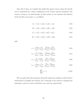
First, the scheduling vector ρ(t) must be specified. For the F-16 aircraft model,
velocity VT and angle of attack α are chosen, which are the most common choices for
the longitudinal motion of an aircraft ([3], [13]). Then, the envelope of interest (call
it ℘ region) is chosen, that is, maximum and minimum values for ρ(t) = [VT , α]T
are
specified.
Let’s consider that
VT,min ≤ VT (t) ≤ VT,max
αmin ≤ α ≤ αmax
and therefore ℘ is a convex region with the following corners (see figure 3.1)
ρ1 = [VT,min αmin]T
ρ2 = [VT,min αmax]T
ρ3 = [VT,max αmax]T
ρ4 = [VT,max αmin]T
The nonlinear model is then linearized around the corner points (that is, linearized
around the trim conditions specified by ρ1, ρ2, ρ3 and ρ4), obtaining 4 different linear
systems with its corresponding state space matrices ([Ai, Bi, Ci, Di] for i = 1, . . . , 4).
38](https://image.slidesharecdn.com/msthesisafarre07-240828145330-68543729/85/MSthesis-control-for-system-s-with-bounded-actuators-pdf-52-320.jpg)
![P4
i=1 τi = τ1 + τ2 + τ3 + τ4 = 1
αa−αb
· 1
Va−Vb
[(αa − αz)(Va − Vz) +
+ (αz − αb)(Va − Vz) + (αz − αb)(Vz − Vb) + (αa − αz)(Vz − Vb)] =
= 1
αa−αb
· 1
Va−Vb
[αaVa − αaVz − αzVa + αzVz + αzVa − αzVz − αbVa +
+ αbVz + αzVz − αzVb − αbVz + αbVb + αaVz − αaVb − αzVz + αzVb] =
= 1
αa−αb
· 1
Va−Vb
[(αa − αb) · (Va − Vb)] = 1
Similarly, it can be shown that on each corner of the LPV region (figure (3.1)) the
value of τi corresponding to that corner is 1 while the rest of them have a 0 value.
To validate this method to obtain an LPV model, we have to compare the behav-
ior of the nonlinear model inside the selected LPV region with the behavior of the
approximated system (3.2)-(3.5). For this validation, we use the same method as in
section 2.4, that is, check the response of both systems to perturbations in the input
commands (δe and T).
To check the region bounded by
160ft/s ≤ VT (t) ≤ 200ft/s (3.11)
32◦
≤ α ≤ 35◦
(3.12)
we simulate the behavior of the nonlinear model in the middle of this zone, that is,
in the trim condition obtained by imposing
VT,Z = 180ft/s (3.13)
αZ = 33.5◦
(3.14)
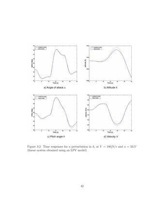
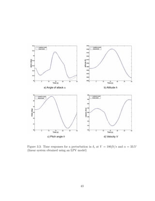
40](https://image.slidesharecdn.com/msthesisafarre07-240828145330-68543729/85/MSthesis-control-for-system-s-with-bounded-actuators-pdf-54-320.jpg)
![and compare it to the behavior of the plant represented in (3.2)-(3.5) with
τ1 = 0.25
τ2 = 0.25
τ3 = 0.25
τ4 = 0.25
Note that this point is located in the middle of the square defined by ρ1, ρ2, ρ3
and ρ4, that is, it corresponds to the point C in figure (3.1). Figures 3.2 and 3.3 show
the results.
We can see that the approximated linear system behaves quite similar to the
nonlinear system, and therefore this method is validated. The same method has
been used to validate the LPV concept in the region bounded by (3.15) and (3.16),
obtaining similar results.
500ft/s ≤ VT (t) ≤ 550ft/s (3.15)
3◦
≤ α ≤ 8◦
(3.16)
It is important, however, to keep in mind the linearization restrictions commented
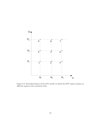
in section 2.4 and also that the LPV region has to be small enough for the method to
be valid. This fact may present a problem: the region may be too small to include the
movements of the aircraft. In other words, if the region defined by the LPV corners
is small, the aircraft may leave it during its trajectory. An option to solve this is to
expand the LPV model as in figure (3.4). Inside each square we use its four corners
to obtain the LPV approximated model, so when the aircraft moves from one square
to the other we just need to change two of the corners and the model will still be
valid [20].
41](https://image.slidesharecdn.com/msthesisafarre07-240828145330-68543729/85/MSthesis-control-for-system-s-with-bounded-actuators-pdf-55-320.jpg)
![Chapter 4
Controller design
4.1 Saturation control background
Actuator saturation has always been a main issue in all engineering fields [9]. It is
probably the most important and dangerous nonlinearity present in any system with
actuators and there are many research projects trying to avoid the problems it causes.
Forgetting to consider it in the controller design can lead to a major degradation of
the system’s performance or, in the worst case, can drive the system unstable (even
for open-loop stable systems).
Saturation occurs often in real life problems because actuators have an inherent
limited capacity and therefore they cannot always provide the action that is required
from them. In other words, actuator saturation means that there is a difference
between the input command to the actuator and its output, that is, when the actuator
reaches its capacity limitation. This limitation can lead to instability.
Equation (4.1) and figure (4.1) show the usual characterization of saturation ef-
fects, being y the actuator input, u the actuator output and umax (umin) the maximum
(minimum) capacity of the actuator.
45](https://image.slidesharecdn.com/msthesisafarre07-240828145330-68543729/85/MSthesis-control-for-system-s-with-bounded-actuators-pdf-59-320.jpg)
![u =
umax if umax ≤ y
y if umin ≤ y < umax
umin if y ≤ umin
(4.1)
Figure 4.1: Plot of the saturation effect
Figure (4.2) shows the scheme of a plant with an open loop controller and a
representation of the actuator. This representation includes a delay (usually due to
mechanical limitations) and a saturation block. This block introduces the saturation
effects described in (4.1). The delay is often modeled as a first order transfer function.
In the flight control world, saturation has been linked to the failure of several
aircrafts [4],[13]. Also, saturation plays a main role in the pilot in-the-loop oscillations
(PIO) [2] and in manual flight control situations, specially in high angle of attack
conditions [4], [15]. Usually, there have been two main approaches to the design of
46](https://image.slidesharecdn.com/msthesisafarre07-240828145330-68543729/85/MSthesis-control-for-system-s-with-bounded-actuators-pdf-60-320.jpg)
![Plant
SATURATION
BLOCK
Controller Delay
Saturation
input
y
Sat.
Output
u
ACTUATOR REPRESENTATION
Figure 4.2: Scheme of a plant with an open loop controller and a representation of
the actuator. The actuator is represented by a saturation block and a delay transfer
function
controllers dealing with saturation.
The first approach takes saturation into account for the design of the controllers
from the beginning of the design process. Usually, this means designing a controller
that is guaranteed not to saturate under any conditions. It is a rather conservative
approach, since the controller will be designed for the worst-case scenario (although
this scenario may never occur) and it involves the combination of various requirements
[10], [17].
The second approach (known as anti-windup) focuses on the design of the best
possible controller even though it may saturate. Once saturation occurs, modifications
to this controller are applied in order to return the system to the non-saturated status.
The main advantage is that is less conservative than the previous method, since a
more aggressive controller is used most of the time. One drawback of this method is
the fact that most anti-windup techniques require an stable open-loop plant, which
is not always the case [4], [14].
For more information on saturation, the reader is referred to [9].
47](https://image.slidesharecdn.com/msthesisafarre07-240828145330-68543729/85/MSthesis-control-for-system-s-with-bounded-actuators-pdf-61-320.jpg)
![4.2 Anti-saturation LMIs: basic equations
Consider the following open loop system
(
ẋ = Ax + B1ω + B2u
z = Cx + D1ω + D2u
(4.2)
where x is the state vector, z is the controlled output, u is the control input and ω is
the disturbance. The state space matrix A can be stable or unstable, depending on
the points about which the model is linearized.
In this thesis only state feedback is considered (4.3), which implies that all the
states can be measured. Assuming that all the states are available is not unusual in
research in flight control [18]. The gain of the controller is represented by K. Using
state feedback, equation (4.2) can be rewritten as (4.4).
u = Kx (4.3)
(
ẋ = (A + B2K)x + B1ω = ACLx + B1ω
z = (C + D2K)x + D1ω
(4.4)
For the disturbance ω, different bounds can be used. In this thesis, we will consider
that we known its peak value (4.5). This is a rather conservative bound, because it
refers to the maximum possible peak value that might occur, but most probably the
disturbance value will be considerably less than this peak value during most or all
of the time. How to reduce this conservatism using a scheduling technique will be
discussed later (section 4.3).
ωT
(t)ω(t) ≤ ω2
max (4.5)
There are three basic constraints to consider when designing controllers that take
saturation nonlinearity into account while responding to a disturbance:
48](https://image.slidesharecdn.com/msthesisafarre07-240828145330-68543729/85/MSthesis-control-for-system-s-with-bounded-actuators-pdf-62-320.jpg)
![where x = (x1, . . . , xN )T
ǫ ℜN
is a vector of unknown variables (the decision or op-
timization variables) and Fi for i = 0, . . . , N are known symmetric matrices. As
long as x enters linearly or affinely in (4.8), the search for a solution is convex. That
means that (4.8) can be solved numerically using very efficiently using optimization
methods, having the guarantee that a solution will be found if it exists.
The importance of Linear Matrix Inequalities and LMI techniques in the control
design area is that a variety of analysis and synthesis problems can be manipulated
until they are in the form of (4.8), or its related form
minimize cT
x subject to F(x) > 0 (4.9)
One example of this manipulation is shown next (corresponds to the basic Lya-
punov stability problem): the system (4.10) is stable if and only if there exists a pos-
itive definite matrix P > 0 such that (4.11) is verified. Equation (4.11) corresponds
to a simple convex search in P, easily done with the software available nowadays.
(
ẋ = Ax
x(0) = x0
(4.10)
PA + AT
P < 0 (4.11)
For more information on LMIs and the software used to solve them, the reader is
referred to [7] [5].
4.2.2 Invariant-set LMI
Remember that we want the state vector to always remain inside an invariant set,
which we define using the ellipsoid ε(P, ωmax) (4.7). This will happen if we can find
a P > 0 such that V̇ ≤ 0 for all states outside of the invariant set. We want to
50](https://image.slidesharecdn.com/msthesisafarre07-240828145330-68543729/85/MSthesis-control-for-system-s-with-bounded-actuators-pdf-64-320.jpg)
![stay inside the invariant set even when there is a perturbation applied to the system,
which can be written mathematically as
V̇ + α(V − ω2
max) < 0 (4.12)
It can be seen that V ≤ ω2
max is an attractive invariant set. The boundary of
the region corresponds to V = ω2
max. Outside this boundary, we’ve got V̇ < 0 and
therefore if you start outside you are attracted to the invariant set. If you are inside,
V̇ can be positive but in the boundary V̇ = 0, which means that we can not leave
the ellipsoid.
So the problem of finding an invariant-set becomes the problem of finding a con-
stant P > 0 matrix (recall that V = xT
Px) that satisfies (4.12). We can rewrite
(4.12) as a linear matrix inequality and then as a matrix expression as follows:
V̇ + α(V − ω2
max) < 0
ẋT
Px + xT
Pẋ + α(xT
Px − ω2
max) < 0
[(A + B2K)x + B1ω]T
Px + xT
P[(A + B2K)x + B1ω] + α(xT
Px − ω2
max) < 0
xT
(AT
P + PA)x + xT
(KT
BT
2 P + PB2K)x + ωT
BT
1 Px + xT
PB1ω − αω2
max < 0
Ã
AT
P + PA + KT
BT
2 P + PB2K + αP PB1
BT
1 P −αI
!
< 0 (4.13)
However, P and K do not show up linearly in the equation (4.13), which makes it
difficult to solve. We can transform it into a convex search by pre and post multiplying
by Ã
P−1
0
0 I
!
51](https://image.slidesharecdn.com/msthesisafarre07-240828145330-68543729/85/MSthesis-control-for-system-s-with-bounded-actuators-pdf-65-320.jpg)
![and by considering
Q = P−1
, F = KQ
The final LMI form of the invariant-set equation is shown in (4.14). This linear
matrix inequality guarantees that the states will remain inside the ellipsoid defined
by P as long as the maximum peak of the disturbance is ω2
max. Given a value for
ω2
max, hence, the objective would be to minimize P such that the value of the control
input is as small as possible (and therefore we avoid saturation).
Ã
(AT
Q + QA + F T
BT
2 + B2F + αQ) B1
BT
1 −αI
!
< 0 (4.14)
4.2.3 Constraint LMI
We do not want the controller to saturate inside the ellipsoid ε(P, ωmax) that defines
the previous invariant set. Mathematically, this condition is expressed by
| u |2
< u2
lim
ω2
max | u |2
< ω2
maxu2
lim
uT ω2
max
u2
lim
u < ω2
max (4.15)
Recalling from the previous sections that V ≤ ω2
max and that u = Kx, we can rewrite
(4.15) in an LMI form:
uT ω2
max
u2
lim
u < V
xT
[KT ω2
max
u2
lim
K]x < xT
Px
KT ω2
max
u2
lim
K < P
52](https://image.slidesharecdn.com/msthesisafarre07-240828145330-68543729/85/MSthesis-control-for-system-s-with-bounded-actuators-pdf-66-320.jpg)
![[ACLx + B1ω]T
Px + xT
P[ACLx + B1ω] − Γ2
ωT
ω +
+ [(C + D2K)x + D1ω]T
[(C + D2K)x + D1ω] < 0 (4.19)
Considering it as a product of a matrix with two vectors and applying the Schur
complement, we get the expression in (4.20). Again, we apply the steps of the end
of section 4.2.2 in order to obtain the final form of the performance linear matrix
inequality (4.21).
P−1
AT
CL + ACLP−1
B1 P−1
(CT
+ KT
DT
2 )
BT
1 −ΓI DT
1
(C + D2K)P−1
D1 −ΓI
< 0 (4.20)
QAT
+ AQ + B2F + F T
BT
2 B1 QCT
+ F T
DT
2
BT
1 −ΓI DT
1
CQ + D2F DT
1 −ΓI
< 0 (4.21)
So, by minimizing the variable Γ we are minimizing the effect of the disturbance
on the controlled output, that is, we are maximizing the performance.
4.3 Scheduling design technique
As mentioned in the previous sections of this chapter, the main problem of considering
the saturation effects at the beginning of the design problem is conservatism, that is,
the obtention of a controller that is valid when the maximum disturbance is applied
but probably will have a poor performance during the rest of the time.
54](https://image.slidesharecdn.com/msthesisafarre07-240828145330-68543729/85/MSthesis-control-for-system-s-with-bounded-actuators-pdf-68-320.jpg)
![In this section, the causes of this conservatism are briefly shown and a gain-
scheduling technique to overcome it is presented. The reader can find detailed expla-
nations of this technique in [17].
4.3.1 Conservatism associated with the design technique
Lets consider that a nominal state-feedback controller Knom is available for the open
loop system (4.22). Also, lets consider that the maximum peak bound value of the
disturbance is known (equation (4.23)). Although it is very unlikely, this maximum
peak value could occur and therefore a controller that does not saturate under ωmax
must be designed.
ẋ = Ax + B1ω + B2u
z = Cx + D1ω + D2u
y = x
(4.22)
ωT
(t)ω(t) ≤ ω2
max (4.23)
Using system analysis LMIs, we can determine the invariant set ellipsoid associ-
ated with ω2
max and Knom, which is ε(Pnom, ωmax) = {x | xT
Pnomx ≤ ω2
max}. This
ellipsoid includes all the possible values that the state vector can take under ω2
max
and the controller Knom. Figure (4.3) shows an scheme of this invariant set ellipsoid
together with the region in which u = Knomx avoids saturation (region between the
parallel lines). Also, a smaller invariant set is shown, which represents the maximum
peak value of the disturbance (ωnom) that Knom can stand without saturating.
The objective is then to design a controller Ksafe that provides a safe override for
the nominal controller. Providing a safe override means that:
- Ksafe does not saturate even for the worst case disturbance
55](https://image.slidesharecdn.com/msthesisafarre07-240828145330-68543729/85/MSthesis-control-for-system-s-with-bounded-actuators-pdf-69-320.jpg)
![−1.5 −1 −0.5 0 0.5 1 1.5
−8
−6
−4
−2
0
2
4
6
8
x
1
x
2
w
max
Linear Region
Linear Region
Linear Region
w
nom
Figure 4.3: Estimate for the smallest invariant set associated with ωmax without
actuator limits (large ellipsoid) and ωnom (small ellipsoid) for Knom. Parallel lines
show region where Knom is not saturated (figure obtained from [17])
- The invariant set associated with Ksafe and ωmax (ε(Psafe, ωmax)) completely
includes the invariant set associated with Knom and ωmax (ε(Pnom, ωmax)), that
is,
Psafe < Pnom (4.24)
Condition (4.24) is necessary because otherwise the state vector may follow some
trajectories which lead outside the safe invariant set (see figure (4.4))and therefore
we have no stability guarantee Ksafe (it may saturate). If we consider Q = P−1
,
condition (4.24) converts into
Qsafe > Qnom (4.25)
Using then LMIs (4.14), (4.16) and (4.21) together with the inclusion condition
(4.25) we obtain a safe controller Ksafe with guarantee that it will not saturate even
for the worst possible disturbance and therefore guaranteeing that the system will
always remain stable.
56](https://image.slidesharecdn.com/msthesisafarre07-240828145330-68543729/85/MSthesis-control-for-system-s-with-bounded-actuators-pdf-70-320.jpg)
![−15 −10 −5 0 5 10 15
−30
−20
−10
0
10
20
30
x
1
x
2
Linear
case
K1
bound
K
1
bound
Figure 4.5: Invariant set associated with ωmax and Ksafe compared to linear case
(figure obtained from [17])
4.3.2 Gain scheduling technique to overcome conservatism
To overcome the conservatism seen in the previous subsection, controller scheduling
is introduced. Consider first a nominal controller (Knom), which in this thesis is
designed solving the following system of LMIs:
AQ + QAT
+ B2Fnom + FT
nomBT
2 B1 QiCT
1 + FT
nomDT
2
BT
1 −ΓiI DT
1
CQ + D2Fnom D1 −ΓiI
(4.26)
Q > 0 (4.27)
Γ > Γmin (4.28)
58](https://image.slidesharecdn.com/msthesisafarre07-240828145330-68543729/85/MSthesis-control-for-system-s-with-bounded-actuators-pdf-72-320.jpg)
![of attack conditions, and therefore it will be considered in this thesis.
To use the controller design method presented in the previous sections, however,
some changes need to be made, because it is based on the disturbance attenuation
problem, not in the tracking one (see section 4.2). To address this problem, we will
use the method proposed in [8], that re-writes the tracking problem in a disturbance
attenuation way by reducing the norm of the error between the tracking signal (ref-
erence) and the controlled output.
As it will be shown next, this method introduces the tracking error into the state
vector and considers the tracking reference as a disturbance. By using L2 gain, it
minimizes the effect of the disturbance on the states, and therefore it minimizes the
tracking error independently of the disturbance (reference signal).
Let’s consider the following system, where xd is the vector we want to track
(reference signal):
˙
x̂ = Âx̂ + B̂2u
ŷ = Cx̂ + D̂12u = [I 0]x̂ = x̂1
e = ŷ − xd = x̂1 − xd
(4.35)
Considering the error as a state,
x̄ =
"
x̂1
x̂2
#
−
"
x̂d
0
#
=
"
x̂1 − x̂d
x̂2
#
=
"
e
x̂2
#
(4.36)
we get the following system
˙
x̄ = Âx̄ + B̂2u −
"
ẋd
0
#
+
"
Â11
Â21
#
xd (4.37)
= Âx̄ + B̂2u +
"
Â11 −I
Â21 0
# "
xd
ẋd
#
(4.38)
= Âx̄ + B̂2u + B̂1ω (4.39)
that has the general form seen in equation (4.2) with the disturbance vector defined
62](https://image.slidesharecdn.com/msthesisafarre07-240828145330-68543729/85/MSthesis-control-for-system-s-with-bounded-actuators-pdf-76-320.jpg)
![as ω = [xd ẋd]T
. Therefore, the maximum peak value for the disturbance can be
defined as
ωT
ω ≤ ω2
max
[xd ẋd]
"
xd
˙
xd
#
≤ ω2
max
x2
d + ẋ2
d ≤ ω2
max
Considering then xd,max and ẋd,max to be the maximum values for xd and ẋd
respectively for all t > 0, we obtain the following estimate for the maximum peak
value:
x2
d,max + ẋ2
d,max ≤ ω2
max (4.40)
63](https://image.slidesharecdn.com/msthesisafarre07-240828145330-68543729/85/MSthesis-control-for-system-s-with-bounded-actuators-pdf-77-320.jpg)
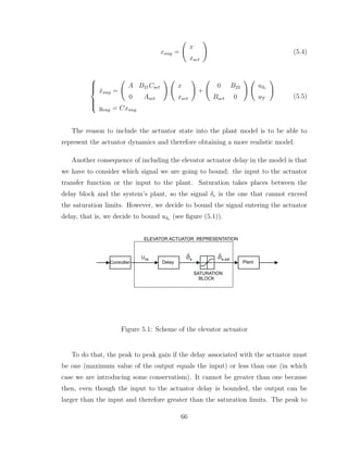
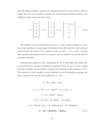
![5.1 Problems setup
In this section we introduce some aspects that required special attention during the
preparation of the aircraft simulations.
5.1.1 Inclusion of the elevator actuator
As explained in the modeling section 2.2.1 (specifically in table (2.2)), the elevator is
considered as a saturation block plus a first order system, which represents the delay
due to physical limitations. The time constant of this first order system is 0.0495 sec
[13] and the corresponding transfer function and state space representation of the
elevator is:
Gact(s) =
20.2
s + 20.2
(5.1)
(
ẋact = Aactxact + B2,actuact = −20.2xact + 20.2uδe
yact = δe = Cactxact = xact
(5.2)
where uδe is the control command referring to the elevator (output of the con-
troller) and δe is the actual input to the aircraft’s plant. Note that the state space
representation has been chosen in order to have δe equal to the state of the actua-
tor. This has been done in order to include the elevator actuator state (xact) in the
aircraft’s state vector, shown next. First, we show the initial aircraft’s plant, then
we change the state vector including xact and finally we show the equations of the
augmented system.
ẋ = Ax + [B21 B22]
Ã
δe
T
!
y = Cx
(5.3)
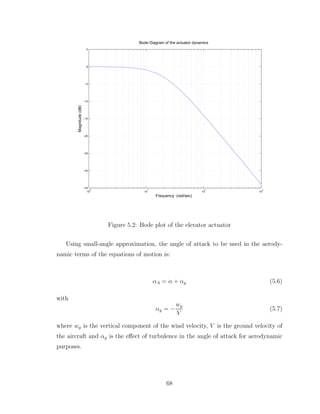
65](https://image.slidesharecdn.com/msthesisafarre07-240828145330-68543729/85/MSthesis-control-for-system-s-with-bounded-actuators-pdf-79-320.jpg)
![peak gain is checked next.
Gact(s) =
20.2
s + 20.2
→ g(t) = 20.2e−20.2t
Peak to peak gain :
R ∞
0
| g(t) | dt =
R ∞
0
20.2e−20.2t
dt
= 20.2 −1
20.2
e−20.2t
|∞
0
= 1.
We can see that the peak to peak gain is 1 and therefore we can limit the signal
before the actuator delay without the risk of getting unstable. However, when check-
ing the Bode plot of the elevator’s transfer function (figure (5.2)) we can see that the
energy gain is 0 dB for low frequencies but it diminishes for higher frequencies. This
means that for higher frequencies the output of the actuator delay is smaller than the
input, and therefore we are adding some conservatism.
5.1.2 Turbulence model for the altitude hold problem
For the first simulation (altitude hold), we need to model the effects of wind distur-
bance. According to [16], the effects of the turbulence are introduced to the equations
of motion of the aircraft by means of its velocity components: longitudinal, horizontal
and vertical. Also according to [16], the effect of the turbulence velocities produces
changes in the aerodynamic forces and moments acting on the airplane. Therefore,
they enter the equations of motion of the aircraft only through the aerodynamic terms
and not the inertial terms.
For altitude hold purposes, the component that mostly affects the response of
the aircraft is the vertical velocity (wg). Since the three gust components can be
considered separately due to the linearity of the system, we will only consider the
vertical component of the gust.
67](https://image.slidesharecdn.com/msthesisafarre07-240828145330-68543729/85/MSthesis-control-for-system-s-with-bounded-actuators-pdf-81-320.jpg)
![The wind turbulence model is obtained from [6]. In the military references, both
the Dryden and the Von Karman spectral representations are used in order to generate
turbulence. Band-limited white noise is filtered by filters derivated from both spectral
representations, obtaining the desired component of the wind turbulence.
In this thesis, the Von Karman representation will be used in order to obtain the
vertical component of the wind turbulence wg. The Von Karman spectra is
Φwg (ω) = σ2
w
Lw
π
1 + 8
3
(1.339Lw
ω
V
)2
[1 + (1.339Lw
ω
V
)2]
11
6
(5.8)
and the continuous filter obtained from it is
Hwg (s) =
σω
q
Lω
V
(1 + 2.7478Lω
V
s + 0.3398(Lω
V
)2
s2
)
1 + 2.9958Lω
V
s + 1.9754(Lω
V
)2s2 + 0.1539(Lω
V
)3s3
(5.9)
where Lw is the scale of vertical turbulence, σw is the vertical gust intensity and
ω is the frequency. For an altitude greater than 2000 ft the length of the vertical
turbulence is Lw = 2500 ft [6].
The turbulence intensities are defined in the diagram shown in figure (5.3) [6].
This diagram shows the probability of exceeding a determinate value of turbulence
amplitude intensity as a function of altitude. For example, for an altitude around
15000 ft there is a slight probability (10−2
) of having a turbulence amplitude larger
than 5 ft/s.
5.1.3 Rearranging the equations for the tracking problem
In order to use the controller design approach to the tracking problem presented in
4.4, the variable that we want to follow the tracking command must be part of the
state vector. The state vector and state space model of the F − 16 that we will
initially consider for the tracking problem is
69](https://image.slidesharecdn.com/msthesisafarre07-240828145330-68543729/85/MSthesis-control-for-system-s-with-bounded-actuators-pdf-83-320.jpg)
![Figure 5.3: Probability of exceedance of turbulence intensity as a function of altitude
(
ẋ = Ax + B2u
y = Cx + D12u
(5.10)
x =
V
α
q
θ
xact
(5.11)
Note that we have incorporated the state of the actuator (as explained in section
5.1.2) and that we no longer consider altitude as a state, which is a common assump-
tion in aircraft tracking problems [13] because its effect on the rest of states is very
small. Also, in the initial simulations altitude remained almost constant so it was
removed from the states for the sake of simplicity of the model.
70](https://image.slidesharecdn.com/msthesisafarre07-240828145330-68543729/85/MSthesis-control-for-system-s-with-bounded-actuators-pdf-84-320.jpg)
![numerical problems too).
To avoid this problem, two changes are introduced in the switching algorithm
shown in section 4.3.2. This changes apply when the system is switching from a low-
gain controller to a higher-gain controller (that is, decreasing i). The reason to apply
this changes only in this case is because when we switch from a high-gain controller
(Khigh) to a lower-gain controller (Klow) we are avoiding the system to saturate, that
is, to leave the corresponding ellipsoid. It is an emergency situation to avoid the
possibility of the system going out of control.
On the contrary, when switching from Klow to a Khigh we are still inside the
ellipsoid associated with the low-gain controller and therefore the system is always
under control. We can delay the switch between the controllers to make sure the
system enters the ellipsoid associated with the higher gain controller instead of the
system getting stuck in the edge of the ellipsoid. Therefore, the objective of the
changes introduced is to delay the switching:
- First, we want to make sure that we switch when the system is inside the higher-
gain ellipsoid instead of just being on the edge. To accomplish this, we reduce
the saturation limit for the higher gain controller when working with the lower
gain one. In other words, instead of switching when Khigh x < 25◦
(for the
elevator) we switch when Khigh x < (25 − ǫ)◦
.
- Second, we want to avoid abrupt changes between controllers. To accomplish
it, we limit the rate of change of the elevator control signal when switching from
Klow to Khigh. We limit this rate as follows (all the matrices and vectors are
available in real time):
u̇ = K ẋ = K [Ax + B2Kx + B1ω] < tan(̺)
In the simulations of this thesis, we used a value of ǫ = 0.5◦
for the elevator and of
ǫ = 100 lb for the thrust. Also, we used a value of ̺ = 86◦
. Taking into account this
changes, the switching algorithms were changed. Next we can see the algorithm used
76](https://image.slidesharecdn.com/msthesisafarre07-240828145330-68543729/85/MSthesis-control-for-system-s-with-bounded-actuators-pdf-90-320.jpg)
![5.2 Altitude hold
The first maneuver that we will use to check the performance of the scheduling con-
troller design technique consists on an altitude hold autopilot. Some examples of
controller design for this autopilot maneuver can be found in [18].
The objective is that the controller must maintain the same altitude independently
of the wind conditions (turbulence). This turbulence basically effects the aerodynamic
coefficients of the airplane, as explained in section 5.1.2 together with the turbulence
model used. According to the design guidelines provided in [18], this altitude hold is
designed also trying to keep the value of θ constant.
The first step is to choose a trim condition in which we want to work. A pilot
usually wants to use the autopilot for altitude hold in cruise flight conditions, that
is, in low angle of attack conditions. It would not make sense to try to keep altitude
constant when flying in a high angle of attack position, mainly because there would
be a huge drag force and it would result in a waste of fuel. The trim condition chosen,
together with the matrices resulting from the linearization and used in the controller
design are shown next.
x0 =
V = 600ft/s
α = 2.68◦
q = 0 rad/s
θ = 2.68◦
h = 20000ft
xact = 0
(5.18)
u0 =
δe = 3.88◦
δptv = 0◦
T = 2207.8 lb
ω = 0 ft/s
(5.19)
78](https://image.slidesharecdn.com/msthesisafarre07-240828145330-68543729/85/MSthesis-control-for-system-s-with-bounded-actuators-pdf-92-320.jpg)
![ẋ = 10−1
−9.968e − 2 −8.378 −7.546 −321.7 1.013e − 3 64.50
−1.778e − 3 −6.502 9.483 0 1.806e − 5 −7.881e − 1
≃ 0 62.84 −6.884 0 ≃ 0 −76.57
0 0 10 0 0 0
≃ 0 −5999 0 5999 0 0
0 0 0 0 0 −202
x +
+ 10−3
1.396
1.084
−1.047
0
0
0
ω +
0
0
0
0
0
20.2
uδe (5.20)
y =
Ã
θ
h
!
=
Ã
0 0 0 1 0 0
0 0 0 0 1 0
!
x (5.21)
This condition is obtained using a relative position of the center of gravity of
xcg = 0.35c̄, which coincides with the reference value xcg,ref = 0.35c̄. This position
is chosen because we assume the aircraft to be on a cruise flight with no changes in
the load that could move the center of gravity from its reference position. Also, in
the altitude hold maneuver only the elevator is considered [18]. We assume that on
a cruise flight the engine is working at the maximum performance level in order to
save fuel and therefore it will not be used to attenuate wind disturbances in order to
keep altitude constant (instead, it would be used to change altitudes for example).
Initially, we check the response of the linear model of the aircraft without any
controller to a moderate disturbance (probability of exceedance of high-altitude in-
tensity = 10e−3
). To obtain the disturbance, a Von Karman wind turbulence model
included in the Simulink Aerospace Blockset r
° is used. The resulting wind veloc-
ity (disturbance signal) and the altitude response are shown in figure (5.5). We can
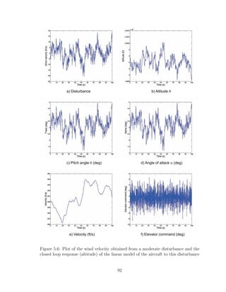
clearly see that the airplane goes unstable, so there is a need of a controller that deals
79](https://image.slidesharecdn.com/msthesisafarre07-240828145330-68543729/85/MSthesis-control-for-system-s-with-bounded-actuators-pdf-93-320.jpg)
![with the wind disturbance applied.
a) Disturbance w b) Altitude h
Figure 5.5: Plot of the wind velocity obtained from a moderate disturbance and the
open loop response (altitude) of the linear model of the aircraft to this disturbance
A very high-gain nominal controller is then designed. Although the values may
be somewhat higher than usual, the objective is to saturate so there is a need for a
safe controller to guarantee stability. Also, in case the safe controller is too conser-
vative the objective is to check the scheduling approach presented in section 4.3.2 to
improve the overall performance of the system. The values of the nominal controller
Knom (obtained using the LMI system (4.26)-(4.28) without taking saturation into
consideration), its performance (Perfnom) and the maximum peak value of the dis-
turbance (ωnom) that it can stand without saturating (theoretically, obtained from
solving the LMIs) are shown in (5.22), (5.23) and (5.24), respectively.
Knom = [ 8.0831 · 10−3
− 299.8368 6.4759 333.4070 1.6589 0 ] (5.22)
Γnom = 0.06244 (5.23)
ωnom = 0.1308 ft/s (5.24)
The response of the aircraft with the nominal controller to the same disturbance
applied before (for a longer period of time, exactly 100 seconds) can be checked in
figure (5.6). Note that the values for the states shown include the trim values of
80](https://image.slidesharecdn.com/msthesisafarre07-240828145330-68543729/85/MSthesis-control-for-system-s-with-bounded-actuators-pdf-94-320.jpg)
![5.3 Tracking
In the previous section we have seen that saturation is not a big issue in the altitude
hold autopilot problem. However, research has been done about saturation of the
actuators of an aircraft during the tracking of trajectories [13]. Therefore, the next
step is to design a tracking maneuver for the flight path angle (γ = θ − α) following
the scheduling design method discussed in 4.3. The changes in the equations in order
to apply this method have been discussed in 4.4 and 5.1.3.
In this tracking problem, altitude will no longer be considered a state of the system
[13]. It will be considered a constant input to the system, and therefore the state
vector from now on is (including the actuator state):
x =
V
α
q
θ
xact
(5.25)
The objective is to track the flight path angle reference command with a maximum
steady state error of 1.25%. This tracking problem is often formulated as a model-
following problem, according to [13], where an ideal second order model is to be
followed,where γcmd is the reference command and γideal is the ideal response that
should be obtained from the aircraft model.
γideal
γcmd
=
w2
ideal
s2 + 2ζidealwideals + w2
ideal
(5.26)
The parameters in 5.26 must be chosen according to the desired flying qualities.
A natural frequency of 1.5rad/s and a damping ratio of 0.8 are chosen [13], obtaining
82](https://image.slidesharecdn.com/msthesisafarre07-240828145330-68543729/85/MSthesis-control-for-system-s-with-bounded-actuators-pdf-96-320.jpg)
![the following ideal model:
γideal
γcmd
=
2.25
s2 + 2.4s + 2.25
(5.27)
The control inputs used for the simulations are the elevator and the engine thrust,
i.e. u = [δe T]T
. The saturation limits for the elevator can be seen in table 2.2.
The saturation limits for the thrust are deduced from the engine model presented in
[18], and presented in table 2.3. Although the engine model shows that the engine
can provide negative thrust, this is only possible in specific conditions: relatively
low altitude (below 30000/; ft), high Mach number (higher than 0.6) and the engine
working on the idle regime. Since during the tracking of a reference flight path angle
the engine is more likely to be working on the military or maximum regime and the
conditions chosen for the simulations have a low Mach number (around 0.1) we will
consider that the engine cannot provide negative thrust, that is, we cannot obtain
negative values for T. Therefore the actual saturation limits for the thrust actuator
are the ones in (5.28).
0 lb ≤ T ≤ 28886 lb (5.28)
The controller design method that we will use requires the setting of the maximum
peak value of the disturbance, for which we will guarantee that the aircraft will not
saturate and will remain stable. The reference signal to track is γideal, which is the
output of the second order system in (5.27). Assuming that the input to this filter is
a step of amplitude A, we can easily obtain the time expression for both γideal and
γ̇ideal and its maximum value given the input step:
γideal = A[1 − e−ξωnt
(cosωdt +
ξ
p
(1 − ξ2)
sinωdt)] (5.29)
˙
γideal = A[sinωdt
ωn
p
1 − ξ2
e−ξωnt
] (5.30)
83](https://image.slidesharecdn.com/msthesisafarre07-240828145330-68543729/85/MSthesis-control-for-system-s-with-bounded-actuators-pdf-97-320.jpg)
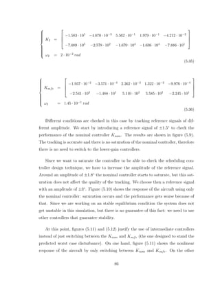
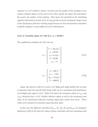
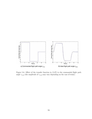
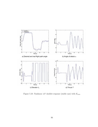
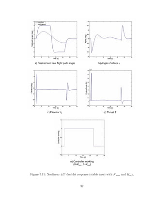
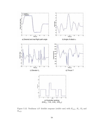
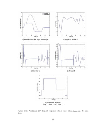
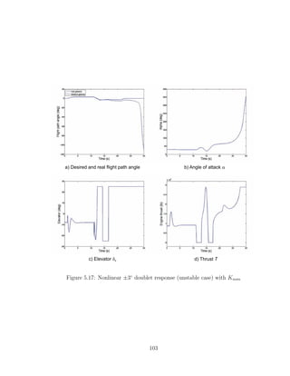
![Two different cases will be shown: an stable and an unstable case. The reason
is to show that this technique can be applied independently of the stability of the
open loop system (which depends on the linearization conditions). In both cases,
the equilibrium conditions have been obtained using a center of gravity position of
xcg = 0.3c̄ (the same one used in [13]) and the nonlinear model has been used in the
simulations. Also, in order to compare the results with [13] a doublet will be used as
the reference signal (γcmd). The response of the second order system (5.27) to this
doublet will be the ideal signal to track (γideal). The differences between γcmd and
γideal can be checked in figure (5.8).
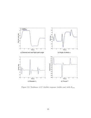
Case 1: Stable plant (V=160 ft/s, α = 35.01◦
)
The equilibrium conditions for this case are:
x0 =
V = 160 ft/s
α = 35.01◦
q = 0 rad/s
θ = 35.01◦
xact = 0
(5.31)
u0 =
h = 3420 ft
δe = −11.31◦
δptv = 0rad/s
T = 10309 lb
(5.32)
In this example the objective will be to track a ±3◦
flight path angle doublet,
although we want to guarantee that the aircraft will remain stable up to a maximum
peak disturbance in the flight path angle of ±5◦
. Table (5.1) shows the maximum
values of γideal and γ̇ideal for a ±5◦
doublet, which are then used to calculate the
maximum peak value of the disturbance/tracking reference signal. These values were
obtained by manually inspecting their plots.
84](https://image.slidesharecdn.com/msthesisafarre07-240828145330-68543729/85/MSthesis-control-for-system-s-with-bounded-actuators-pdf-98-320.jpg)
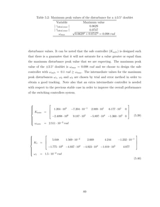
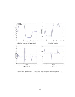
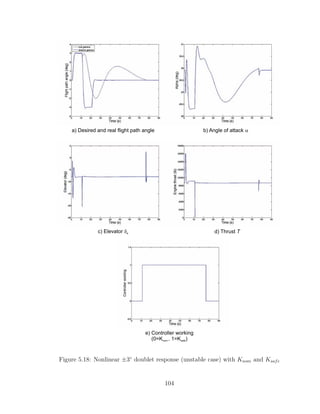
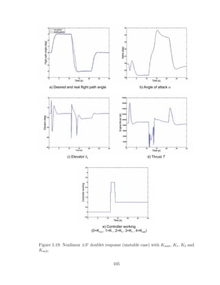
![hand, figure (5.12) shows the nonlinear response by using the 4 controllers introduced
before (the variable controller on the bottom plot shows which controller is active,
i.e. the non saturated controller with a higher gain). Although saturation does not
occur in any of the two situations, it can be clearly seen that the tracking in the
second situation is much better than in the first one, which is the key aspect of this
new technique being tested.
In the first situation, only the nominal controller and the safe controller are avail-
able, therefore when the nominal controller saturates we must switch to the safe
controller, no matter the level of the disturbance and if the nominal controller is
highly or just slightly saturated. This controller has a low gain and its performance
is not optimal, since it is designed to guarantee stability even for the worst-case sce-
nario and in that case performance is not the main concern. Instead, in the second
situation we do not have to only switch between the nominal and the safe controller
because there are the intermediate controllers also available. These controllers are
designed considering different levels of disturbance, and have intermediate gains and
performances between the nominal and the safe controller. For a low level of dis-
turbance we can continue using high gain controllers (e.g. K1 or K2) with a very
good performance while we still have the safe controller on top of them to guarantee
stability in case the worst-case scenario shows up.
Finally, figure (5.13) shows the response of the nonlinear aircraft to a ±5◦
doublet
as the reference flight path angle, which is the worst-case scenario considered in the
controller design. The objective is to show that stability is guaranteed even in this
worst-case scenario, although the tracking is not optimal. However, this is not a big
concern since the priority in a high angle of attack situation is to guarantee stability
and not tracking quality, which is a priority in the low angle of attack region [19].
The results from [13] in the same equilibrium condition can be seen in figures
(5.14) and (5.15) in order to compare them with the results from this thesis. It can
be seen that when the tracking signal has a small amplitude (±1◦
doublet in [13],
±1.5◦
in this thesis) the nominal controllers do not saturate and the performances are
practically the same (compare figures (5.9) and (5.14)). Then a ±2◦
doublet is used in
[13] to check the performance of their anti-windup controller, while in this thesis the
87](https://image.slidesharecdn.com/msthesisafarre07-240828145330-68543729/85/MSthesis-control-for-system-s-with-bounded-actuators-pdf-101-320.jpg)
![Figure 5.14: For comparison purposes: nonlinear ±1◦
doublet response (stable case)
with an LTI nominal controller (extracted from [13])
100](https://image.slidesharecdn.com/msthesisafarre07-240828145330-68543729/85/MSthesis-control-for-system-s-with-bounded-actuators-pdf-114-320.jpg)
![Figure 5.15: For comparison purposes: nonlinear ±2◦
doublet response (stable case)
with/without an LTI antiwindup compensator (extracted from [13])
101](https://image.slidesharecdn.com/msthesisafarre07-240828145330-68543729/85/MSthesis-control-for-system-s-with-bounded-actuators-pdf-115-320.jpg)

![Chapter 6
Conclusions
The structure of this study has mainly followed the structure of [13] to be able to
qualitatively compare the results obtained using a regular anti-windup approach and
the new technique combining both anti-windup and direct approach methods.
The nonlinear longitudinal model of an F − 16 aircraft has been developed and
implemented in this thesis. Although it has not been used, the model includes the
possibility to vector the thrust, which probably can improve the performance of the
aircraft in the high angle of attack region. To be able to use linear techniques in the
design of the controller, this model has been linearized and validated about different
equilibrium conditions. The results of the validation process showed that the linear
model is a good representation of the nonlinear model as long as changes in the
aerodynamic behavior of the aircraft are small, that is, as long as changes in the
angle of attack are small and the aircraft stays outside the transient region between
low and high angle of attack behavior (around 20◦
).
The main problem of using linear methods to design the controllers is that they will
only work while the linear model accurately represents the real nonlinear model, which
is basically in a small region about the equilibrium condition used in the linearization
process. This drawback is especially important in flight control system design since
107](https://image.slidesharecdn.com/msthesisafarre07-240828145330-68543729/85/MSthesis-control-for-system-s-with-bounded-actuators-pdf-121-320.jpg)
![results (exaggerated velocity of the wind). This case was then dropped in order to
focus the efforts on the tracking case.
The results on the tracking case have been very positive. The anti-windup con-
cept included in the combined technique allows the nominal controller to work most
of the time, since we do not switch until it is saturated. Given the fact that this
controller has the desired performance and properties, the more we use it the better
the overall performance. Also, the scheduling concept has been very useful to improve
the overall performance of the system, since it allowed to use more aggressive con-
trollers depending on the level of the disturbance instead of just using a low-gain safe
controller anytime that the nominal controller was saturated. The results obtained
from the stable case can be compared to the ones in [13] showing a similar degree of
performance. In addition, using this technique has allowed us to check an unstable
case showing that the results are also quite desirable.
Further work in this area would be to use output feedback instead of state feed-
back, which would take into account that not all the states of the system may be
available. In addition, using output feedback would allow to consider also rate limits
in the controller signal, specially important since the results obtained in this thesis
show steep command signals that may be problematic when considering rate satura-
tion.
109](https://image.slidesharecdn.com/msthesisafarre07-240828145330-68543729/85/MSthesis-control-for-system-s-with-bounded-actuators-pdf-123-320.jpg)
![Bibliography
[1] Francesco Amato. Robust Control of Linear Systems Subject to Uncertain Time-
Varying Parameters. Springer, first edition, 2005.
[2] Francesco Amato, Raffaele Iervolino, Stefano Scala, and Leopoldo Verde. Cate-
gory ii pilot-in-the-loop oscillations analysis from robust stability methods. Jour-
nal of Guidance, Control and Dynamics, pages 531–538, 2001.
[3] Gary Balas and Andres Marcos. Linear parameter varying modeling of the boeing
747-100/200 longitudinal motion. AIAA Guidance, Navigation, and Control
Conference and Exhibit, Montreal, Canada, 2001.
[4] C. Barbu, R. Reginatto, A.R. Teel, and L. Zaccarian. Anti-windup design for
manual flight control. Proceedings of the American Control Conference San
Diego, California, 1999.
[5] Stephen Boyd, Laurent El Ghaoui, Eric Feron, and Venkataramanan Balakr-
ishnan. Linear Matrix Inequalities in System and Control Theory. Society for
Industrial and Applied Mathematics (SIAM), first edition, 1994.
[6] Stacey Gage. Creating a unified graphical wind turbulence model from multiple
specifications. AIAA Modeling and Simulation Technologies Conference and
Exhibit, Austin, TX, 2003.
[7] Pascal Gahinet, Arkadi Nemirovski, Alan J. Laub, and Mahmoud Chilali. LMI
Control Toolbox, first edition, 1995.
110](https://image.slidesharecdn.com/msthesisafarre07-240828145330-68543729/85/MSthesis-control-for-system-s-with-bounded-actuators-pdf-124-320.jpg)
![[8] Faryar Jabbari and Jin-Hoon Kim. A scheduling approach for tracking of general
signals. 2006.
[9] Vikram Kapila and Karolos M. Grigoriadis et altri. Actuator Saturation Control.
Control Engineering Series, first edition, 2002.
[10] Emre Köse and Faryar Jabbari. Scheduled controller for linear systems with
bounded actuators. Automatica, 39:1377–1387, 2003.
[11] I. Emre Köse. Parameter-varying control techniques applied to nonlinear sys-
tems: a general framework. 2000.
[12] Nguyen L.T., Ogburn M.E., Gillert W.P., and et altri. Simulator study of
stall/post-stall characteristics of a fighter airplane with relaxed longitudinal
static stability. NASA Technical Paper 1538, 1979.
[13] Bei Lu. Linear Parameter-Varying Control of An F-16 Aircraft at High Angle of
Attack. PhD thesis, North Carolina State University, 2004.
[14] Eric F. Mulder, Mayuresh V. Kothare, and Manfred Morari. Multivariable anti-
windup controller synthesis using linear matrix inequalities. Automatica, pages
1407–1416, 2001.
[15] William C. Reigelsperger and Siva S. Banda. Nonlinear simulation of a modified
f-16 with full-envelope control laws. Control Engineering Practice, pages 309–320,
1998.
[16] Jan Roskam. Airplane flight dynamics and automatic flight controls. Roskam
Aviation and Engineering Corporation, first edition, 1979.
[17] Solmaz Sajjadi-Kia and Faryar Jabbari. Use of scheduling for anti-windup con-
troller design. 2007.
[18] Brian L. Stevens and Frank L. Lewis. Aircraft Control and Simulation. John
Wiley and Sons INC., second edition, 2003.
[19] Fen Wu, Ashok Gopalarathnam, and Sungwan Kim. Post-stall aerodynamic
modeling and gain-scheduled control design. AIAA Guidance, Navigation, and
Control Conference and Exhibit, San Francisco, CA, 2005.
111](https://image.slidesharecdn.com/msthesisafarre07-240828145330-68543729/85/MSthesis-control-for-system-s-with-bounded-actuators-pdf-125-320.jpg)
![[20] Zhongwei Yu, Huitang Chen, and Peng yung Woo. Gain scheduled linear pa-
rameter varying h∞ control based on lmi approach for a robotic manipulator.
Journal of Robotic Systems, pages 585–593, 2002.
112](https://image.slidesharecdn.com/msthesisafarre07-240828145330-68543729/85/MSthesis-control-for-system-s-with-bounded-actuators-pdf-126-320.jpg)