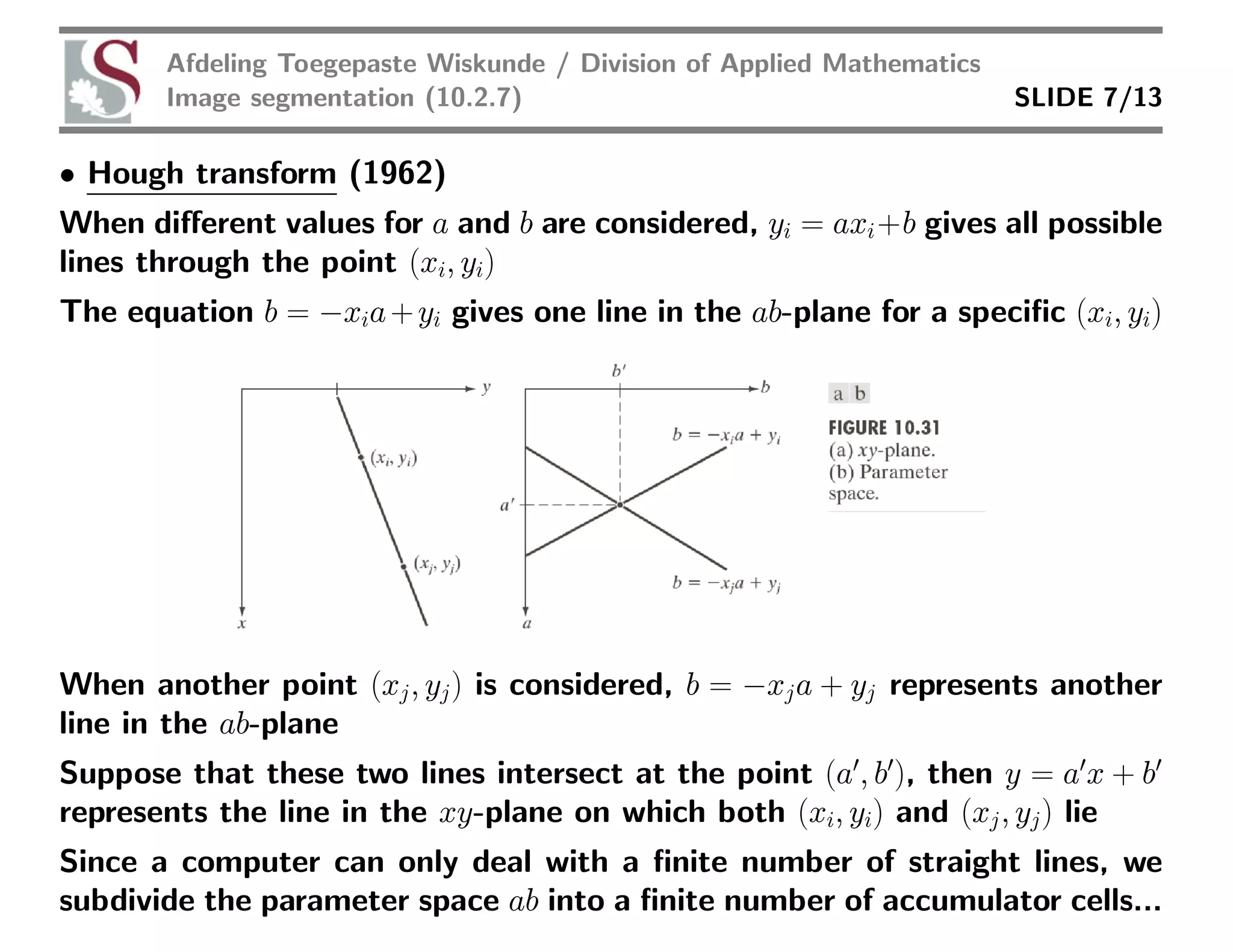
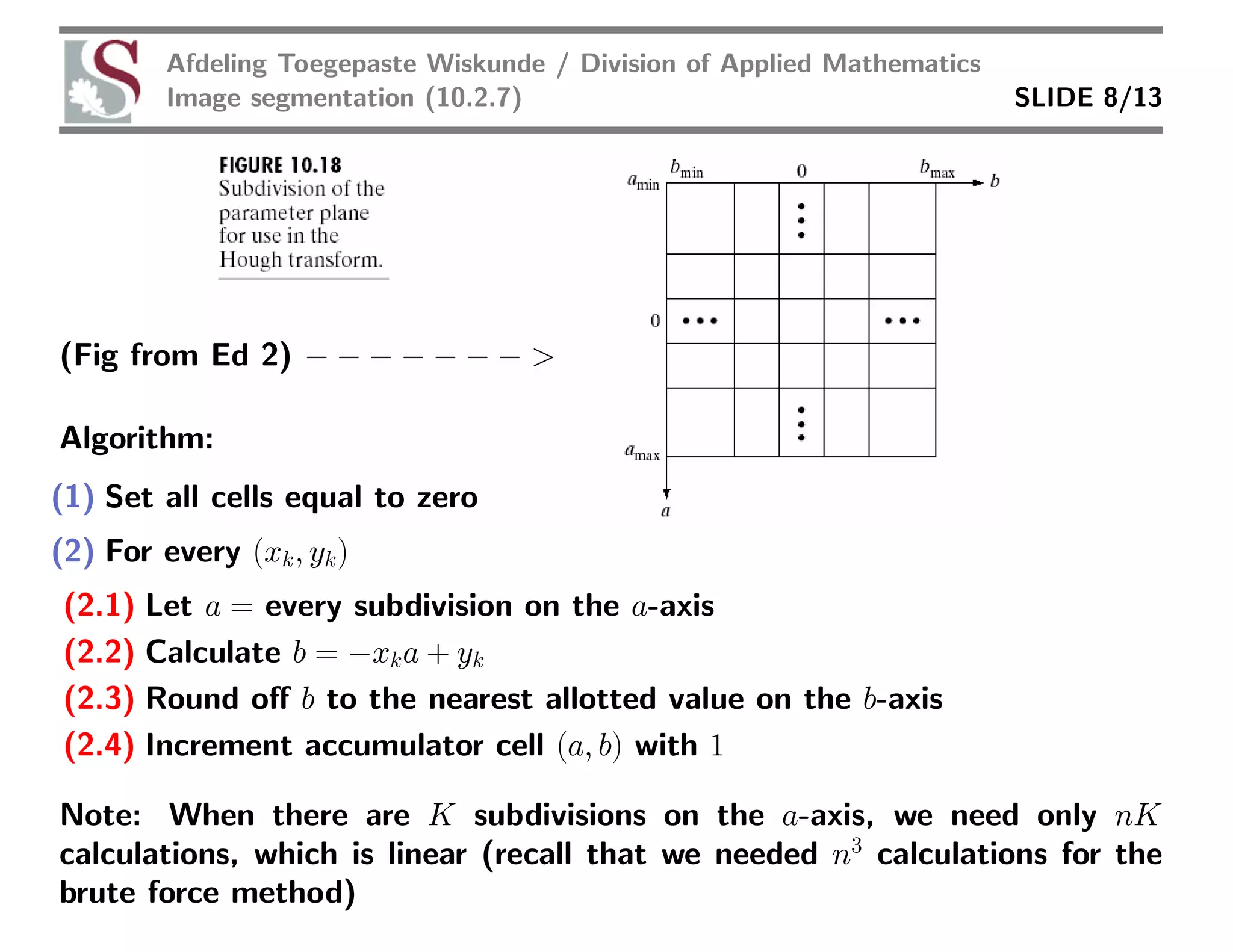
Afdeling Toegepaste Wiskunde / Division of Applied Mathematics
Image segmentation (10.2.7) SLIDE 1/13
10.2.7 Edge linking and boundary detection
Edge detection is always followed by edge linking
Local processing
• Analyze pixels in small neighbourhood Sxy of each edge point
• Pixels that are similar are linked
• Principal properties used for establishing similarity:
(1) M(x, y) = |∇f(x, y)|: Magnitude of gradient vector
(2) α(x, y): Direction of gradient vector
• Edge pixel with coordinates (s, t) in Sxy is similar in magnitude to pixel at
(x, y) if
|M(s, t) − M(x, y)| < E
• Edge pixel with coordinates (s, t) in Sxy has an angle similar to pixel at
(x, y) if
|α(s, t) − α(x, y)| < A
• Edge pixel (s, t) in Sxy is linked with (x, y) if both criteria are satisfied
Afdeling Toegepaste Wiskunde / Division of Applied Mathematics
Image segmentation (10.2.7) SLIDE 2/13
The above strategy is expensive. A record has to be kept of all linked points
by, for example, assigning a different label to every set of linked points
Simplification suitable for real-time applications:
(1) Compute M(x, y) and α(x, y) of input image f(x, y)
(2) Form binary image
g(x, y) =

1, if M(x, y)  TM AND α(x, y) ∈ [A − TA, A + TA]
0, otherwise
(3) Scan rows of g and fill (set to 1) all gaps (sets of 0s) in each row that
do not exceed a specified length K
(4) Rotate g by θ and apply step (3). Rotate result back by −θ.
Image rotation is expensive ⇒ when linking in numerous directions is re-
quired, steps (3) and (4) are combined into a single, radial scanning proce-
dure.
Afdeling Toegepaste Wiskunde / Division of Applied Mathematics
Image segmentation (10.2.7) SLIDE 3/13
Example 10.10:
Afdeling Toegepaste Wiskunde / Division of Applied Mathematics
Image segmentation (10.2.7) SLIDE 4/13
Regional processing (Polygonal approximations)
A conceptual understanding of this idea is sufficient
Requirements: (1) Two starting points must be specified; (2) All the points
must be ordered
Large distance between successive points, relative to the distance between
other points ⇒ boundary segment (open curve) ⇒ end points used as start-
ing points
Seperation between points uniform ⇒ boundary (closed curve) ⇒ extreme
points used as starting points
Afdeling Toegepaste Wiskunde / Division of Applied Mathematics
Image segmentation (10.2.7) SLIDE 5/13
Example 10.11: Edge linking using polygonal approximation
Example 10.12: (READ)
Afdeling Toegepaste Wiskunde / Division of Applied Mathematics
Image segmentation (10.2.7) SLIDE 6/13
Global Processing using the Hough transform
• We attempt to link edge pixels that lie on specified curves
• Brute force method:
When the specified curve is a straight line, the line between each pair of
edge pixels in the image is considered. The distance between every other
edge pixel and the line in question is then calculated.
When the distance is less than a specified threshold, the pixel is considered
to be part of the line
Number of calculations for n edge pixels:
Number of possible lines:
n−1
k=1 k = n(n−1)
2 ≈ n2
Distances per line: n
Total number of distances: n2(n−1)
2 ≈ n3
When n = 2562
then number of calculations is 1.4 × 10¹⁴
!!!
Afdeling Toegepaste Wiskunde / Division of Applied Mathematics
Image segmentation (10.2.7) SLIDE 7/13
• Hough transform (1962)
When different values for a and b are considered, yi = axi+b gives all possible
lines through the point (xi, yi)
The equation b = −xia+yi gives one line in the ab-plane for a specific (xi, yi)
When another point (xj, yj) is considered, b = −xja + yj represents another
line in the ab-plane
Suppose that these two lines intersect at the point (a′
, b′
), then y = a′
x + b′
represents the line in the xy-plane on which both (xi, yi) and (xj, yj) lie
Since a computer can only deal with a finite number of straight lines, we
subdivide the parameter space ab into a finite number of accumulator cells...
Afdeling Toegepaste Wiskunde / Division of Applied Mathematics
Image segmentation (10.2.7) SLIDE 8/13
(Fig from Ed 2) − − − − − − − 
Algorithm:
(1) Set all cells equal to zero
(2) For every (xk, yk)
(2.1) Let a = every subdivision on the a-axis
(2.2) Calculate b = −xka + yk
(2.3) Round off b to the nearest allotted value on the b-axis
(2.4) Increment accumulator cell (a, b) with 1
Note: When there are K subdivisions on the a-axis, we need only nK
calculations, which is linear (recall that we needed n3
calculations for the
brute force method)
Afdeling Toegepaste Wiskunde / Division of Applied Mathematics
Image segmentation (10.2.7) SLIDE 9/13
We still have a problem though, since −∞  a  ∞ and −∞  b  ∞!
In order to deal with this problem, we now represent a straight line as follows
x cos θ + y sin θ = ρ
so that (a, b) → (ρ, θ)
Afdeling Toegepaste Wiskunde / Division of Applied Mathematics
Image segmentation (10.2.7) SLIDE 10/13
Derivation: y = ax + b
b
ρ
= csc θ =
1
sin θ
b = ρ csc θ
a = −
1
tan θ
(negative reciprocal)
= −
cos θ
sin θ
y = −
cos θ
sin θ
x + ρ csc θ ⇒ y sin θ = −x cos θ + ρ ⇒ x cos θ + y sin θ = ρ
Now we have that ρ ∈ [−
√
2D,
√
2D] and θ ∈ [−90o, 90o], where
√
2D is
the diagonal distance between two opposite corners in the image. Problem
solved!
Algorithm:
(1) Set all cells equal to zero
(2) For every (xk, yk)
(2.1) Let θ = every subdivision on the θ-axis
(2.2) Calculate ρ = xk cos θ + yk sin θ
(2.3) Round off ρ to the nearest allotted value on the ρ-axis
(2.4) Increment accumulator cell (ρ, θ) with 1
Afdeling Toegepaste Wiskunde / Division of Applied Mathematics
Image segmentation (10.2.7) SLIDE 11/13
Example 10.13: Illustration of Hough transform properties
Afdeling Toegepaste Wiskunde / Division of Applied Mathematics
Image segmentation (10.2.7) SLIDE 12/13
Algorithm for edge linking:
(1) Compute |∇f| and isolate edge pixels through thresholding
(2) Specify subdivisions in the ρθ-plane
(3) Apply Hough transform to edge pixels
(4) Identify accumulator cells with highest values
(5) Examine continuity of pixels that constitute cell
(6) Link these pixels if gaps are smaller than threshold
Extension to more general graphs
• Hough transform applicable to any graph g(v, c) = 0, where v is vector of
coordinates and c is vector of coefficients
• Example: Find the points that lie on a circle
(x − c1)2
+ (y − c2)2
= c2
3
The presence of three parameters (c1, c2 and c3) results in a 3-D parameter
space with cubelike cells and accumulators of the form A(i, j, k)!
Afdeling Toegepaste Wiskunde / Division of Applied Mathematics
Image segmentation (10.2.7) SLIDE 13/13
Example 10.14: Using the Hough transform for edge linking

Edge linking hough transform

  • 1.
    Afdeling Toegepaste Wiskunde/ Division of Applied Mathematics Image segmentation (10.2.7) SLIDE 1/13 10.2.7 Edge linking and boundary detection Edge detection is always followed by edge linking Local processing • Analyze pixels in small neighbourhood Sxy of each edge point • Pixels that are similar are linked • Principal properties used for establishing similarity: (1) M(x, y) = |∇f(x, y)|: Magnitude of gradient vector (2) α(x, y): Direction of gradient vector • Edge pixel with coordinates (s, t) in Sxy is similar in magnitude to pixel at (x, y) if |M(s, t) − M(x, y)| < E • Edge pixel with coordinates (s, t) in Sxy has an angle similar to pixel at (x, y) if |α(s, t) − α(x, y)| < A • Edge pixel (s, t) in Sxy is linked with (x, y) if both criteria are satisfied
  • 2.
    Afdeling Toegepaste Wiskunde/ Division of Applied Mathematics Image segmentation (10.2.7) SLIDE 2/13 The above strategy is expensive. A record has to be kept of all linked points by, for example, assigning a different label to every set of linked points Simplification suitable for real-time applications: (1) Compute M(x, y) and α(x, y) of input image f(x, y) (2) Form binary image g(x, y) = 1, if M(x, y) TM AND α(x, y) ∈ [A − TA, A + TA] 0, otherwise (3) Scan rows of g and fill (set to 1) all gaps (sets of 0s) in each row that do not exceed a specified length K (4) Rotate g by θ and apply step (3). Rotate result back by −θ. Image rotation is expensive ⇒ when linking in numerous directions is re- quired, steps (3) and (4) are combined into a single, radial scanning proce- dure.
  • 3.
    Afdeling Toegepaste Wiskunde/ Division of Applied Mathematics Image segmentation (10.2.7) SLIDE 3/13 Example 10.10:
  • 4.
    Afdeling Toegepaste Wiskunde/ Division of Applied Mathematics Image segmentation (10.2.7) SLIDE 4/13 Regional processing (Polygonal approximations) A conceptual understanding of this idea is sufficient Requirements: (1) Two starting points must be specified; (2) All the points must be ordered Large distance between successive points, relative to the distance between other points ⇒ boundary segment (open curve) ⇒ end points used as start- ing points Seperation between points uniform ⇒ boundary (closed curve) ⇒ extreme points used as starting points
  • 5.
    Afdeling Toegepaste Wiskunde/ Division of Applied Mathematics Image segmentation (10.2.7) SLIDE 5/13 Example 10.11: Edge linking using polygonal approximation Example 10.12: (READ)
  • 6.
    Afdeling Toegepaste Wiskunde/ Division of Applied Mathematics Image segmentation (10.2.7) SLIDE 6/13 Global Processing using the Hough transform • We attempt to link edge pixels that lie on specified curves • Brute force method: When the specified curve is a straight line, the line between each pair of edge pixels in the image is considered. The distance between every other edge pixel and the line in question is then calculated. When the distance is less than a specified threshold, the pixel is considered to be part of the line Number of calculations for n edge pixels: Number of possible lines: n−1 k=1 k = n(n−1) 2 ≈ n2 Distances per line: n Total number of distances: n2(n−1) 2 ≈ n3 When n = 2562 then number of calculations is 1.4 × 10¹⁴ !!!
  • 7.
    Afdeling Toegepaste Wiskunde/ Division of Applied Mathematics Image segmentation (10.2.7) SLIDE 7/13 • Hough transform (1962) When different values for a and b are considered, yi = axi+b gives all possible lines through the point (xi, yi) The equation b = −xia+yi gives one line in the ab-plane for a specific (xi, yi) When another point (xj, yj) is considered, b = −xja + yj represents another line in the ab-plane Suppose that these two lines intersect at the point (a′ , b′ ), then y = a′ x + b′ represents the line in the xy-plane on which both (xi, yi) and (xj, yj) lie Since a computer can only deal with a finite number of straight lines, we subdivide the parameter space ab into a finite number of accumulator cells...
  • 8.
    Afdeling Toegepaste Wiskunde/ Division of Applied Mathematics Image segmentation (10.2.7) SLIDE 8/13 (Fig from Ed 2) − − − − − − − Algorithm: (1) Set all cells equal to zero (2) For every (xk, yk) (2.1) Let a = every subdivision on the a-axis (2.2) Calculate b = −xka + yk (2.3) Round off b to the nearest allotted value on the b-axis (2.4) Increment accumulator cell (a, b) with 1 Note: When there are K subdivisions on the a-axis, we need only nK calculations, which is linear (recall that we needed n3 calculations for the brute force method)
  • 9.
    Afdeling Toegepaste Wiskunde/ Division of Applied Mathematics Image segmentation (10.2.7) SLIDE 9/13 We still have a problem though, since −∞ a ∞ and −∞ b ∞! In order to deal with this problem, we now represent a straight line as follows x cos θ + y sin θ = ρ so that (a, b) → (ρ, θ)
  • 10.
    Afdeling Toegepaste Wiskunde/ Division of Applied Mathematics Image segmentation (10.2.7) SLIDE 10/13 Derivation: y = ax + b b ρ = csc θ = 1 sin θ b = ρ csc θ a = − 1 tan θ (negative reciprocal) = − cos θ sin θ y = − cos θ sin θ x + ρ csc θ ⇒ y sin θ = −x cos θ + ρ ⇒ x cos θ + y sin θ = ρ Now we have that ρ ∈ [− √ 2D, √ 2D] and θ ∈ [−90o, 90o], where √ 2D is the diagonal distance between two opposite corners in the image. Problem solved! Algorithm: (1) Set all cells equal to zero (2) For every (xk, yk) (2.1) Let θ = every subdivision on the θ-axis (2.2) Calculate ρ = xk cos θ + yk sin θ (2.3) Round off ρ to the nearest allotted value on the ρ-axis (2.4) Increment accumulator cell (ρ, θ) with 1
  • 11.
    Afdeling Toegepaste Wiskunde/ Division of Applied Mathematics Image segmentation (10.2.7) SLIDE 11/13 Example 10.13: Illustration of Hough transform properties
  • 12.
    Afdeling Toegepaste Wiskunde/ Division of Applied Mathematics Image segmentation (10.2.7) SLIDE 12/13 Algorithm for edge linking: (1) Compute |∇f| and isolate edge pixels through thresholding (2) Specify subdivisions in the ρθ-plane (3) Apply Hough transform to edge pixels (4) Identify accumulator cells with highest values (5) Examine continuity of pixels that constitute cell (6) Link these pixels if gaps are smaller than threshold Extension to more general graphs • Hough transform applicable to any graph g(v, c) = 0, where v is vector of coordinates and c is vector of coefficients • Example: Find the points that lie on a circle (x − c1)2 + (y − c2)2 = c2 3 The presence of three parameters (c1, c2 and c3) results in a 3-D parameter space with cubelike cells and accumulators of the form A(i, j, k)!
  • 13.
    Afdeling Toegepaste Wiskunde/ Division of Applied Mathematics Image segmentation (10.2.7) SLIDE 13/13 Example 10.14: Using the Hough transform for edge linking