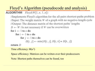
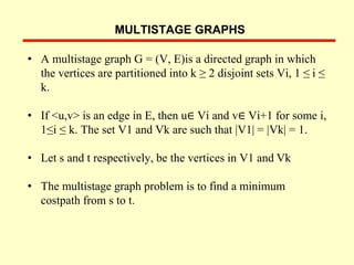
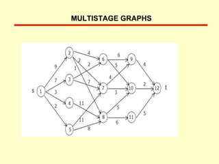
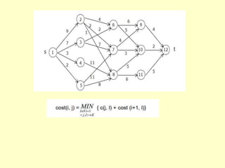
The document describes several algorithms that use dynamic programming techniques. It discusses the coin changing problem, computing binomial coefficients, Floyd's algorithm for finding all-pairs shortest paths, optimal binary search trees, the knapsack problem, and multistage graphs. For each problem, it provides the key recurrence relation used to build the dynamic programming solution in a bottom-up manner, often using a table to store intermediate results. It also analyzes the time and space complexity of the different approaches.

1. DESIGN AND ANALYSIS
OF ALGORITHMS
DYNAMIC PROGRAMMING TECHNIQUE

2. • Coin changing problem
• Computing a Binomial Coefficient
• Floyd‘s algorithm
• Multi stage graph
• Optimal Binary Search Trees
• Knapsack Problem and Memory functions.
Contents

3. Dynamic Programming is a general algorithm design technique
for solving problems defined by recurrences with overlapping
subproblems
• Invented by American mathematician Richard Bellman in the 1950s to
solve optimization problems and later assimilated by CS
• “Programming” here means “planning”
• Main idea:
-set up a recurrence relating a solution to a larger instance to
solutions of some smaller instances
- solve smaller instances once
-record solutions in a table
-extract solution to the initial instance from that table
Dynamic Programming

4. Computing the nth Fibonacci number using bottom-up iteration and recording
results:
F(0) = 0
F(1) = 1
F(2) = 1+0 = 1
…
F(n-2) =
F(n-1) =
F(n) = F(n-1) + F(n-2)
Efficiency:
- time
- space
Fibonacci numbers

5. • Input: A list of integers representing coin
denominations, plus another positive integer
representing an amount of money.
• Output: A minimal collection of coins of the given
denominations which sum to the given amount.
• Give change for amount n using the minimum
number of coins of denominations d1<d2 < . . .<dm.
Coin-changing problem

6. Example : amount n = 6 and coin
denominations 1, 3, and 4.
Coin-changing problem

7. .
Coin-changing problem

8. Binomial coefficient, denoted c(n,k), is the number of
combinations k elements from an n-element set (0 ≤ k ≤ n).
The binomial formula is:
(a+b)n = c(n,0)an + …. + c(n,i)a n-i b i + … + c(n,n)bn
c(n,k) = c(n-1,k-1) + c(n-1,k) for n>k>0
and
c(n,0)= c(n,n) = 1
COMPUTING A BINOMIAL COEFFICIENT

9. c(n,k) = c(n-1,k-1) + c(n-1,k) for n>k>0
and c(n,0)= c(n,n) = 1
COMPUTING A BINOMIAL COEFFICIENT

10. COMPUTING A BINOMIAL COEFFICIENT
Analysis:
Time efficiency: Θ(nk)
Space efficiency: Θ(nk)

11. Given n items of
integer weights: w1 w2 … wn
values: v1 v2 … vn
a knapsack of integer capacity W
find most valuable subset of the items that fit into the knapsack
Recursive solution?
What is smaller problem?
How to use solution to smaller in solution to larger
Table?
Order to solve?
Initial conditions?
Knapsack Problem by DP

12. Example: Knapsack of capacity W = 5
item weight value
1 2 $12
2 1 $10
3 3 $20
4 2 $15
Knapsack Problem by DP (example)

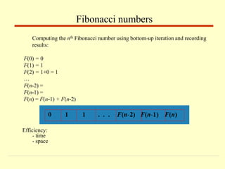
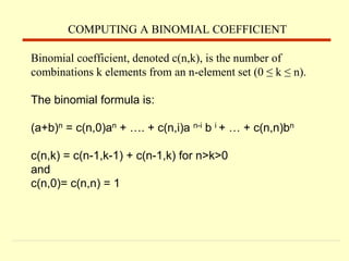
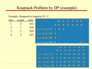
13. Given n items of
integer weights: w1 w2 … wn
values: v1 v2 … vn
a knapsack of integer capacity W
find most valuable subset of the items that fit into the knapsack
Consider instance defined by first i items and capacity j (j  W).
Let V[i,j] be optimal value of such instance. Then
max {V[i-1,j], vi + V[i-1,j- wi]} if j- wi  0
V[i,j] =
V[i-1,j] if j- wi < 0
Initial conditions: V[0,j] = 0 and V[i,0] = 0
Knapsack Problem by DP

14. Problem: Given n keys a1 < …< an and probabilities p1 ≤ … ≤
pn
searching for them, find a BST with a minimum
average number of comparisons in successful search.
Since total number of BSTs with n nodes is given by
C(2n,n)/(n+1), which grows exponentially, brute force is
hopeless.
Optimal Binary Search Trees

15. Example: What is an optimal BST for keys A, B, C, and D with
search probabilities 0.1, 0.2, 0.4, and 0.3,
respectively?
Optimal Binary Search Trees
Example: key A B C D
probability 0.1 0.2 0.4 0.3
B
A
C
D
Optimal BST

16. Expected number of comparisons for optimal BST:
1*0.4 + 2*(0.2+0.3) + 3*(0.1) = 0.4+1.0+0.3=1.7
Non-optimal BST – Swap A and B:
1*0.4 + 2*(0.1+0.3) + 3*(0.2) = 0.4+0.8+0.6=1.8
Optimal Binary Search Trees
B
A
C
D
Example: key A B C D
probability 0.1 0.2 0.4 0.3

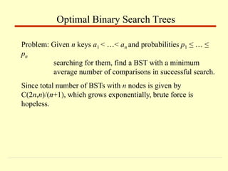
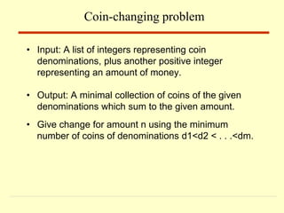
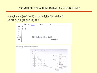
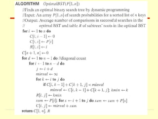
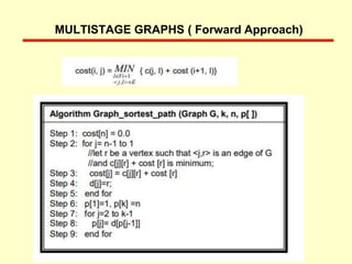
17. After simplifications, we obtain the recurrence for C[i,j]:
C[i,j] = min {C[i,k-1] + C[k+1,j]} + ∑ ps for 1 ≤ i ≤ j ≤ n
C[i,i] = pi for 1 ≤ i ≤ j ≤ n
DP for Optimal BST Problem (cont.)
goal
0
0
C[i,j]
0
1
n+1
0 1 n
p 1
p2
n
p
i
j

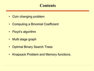
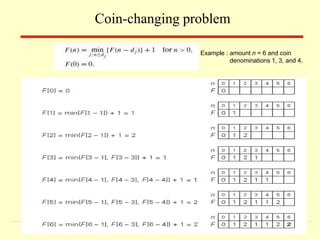
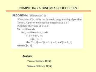
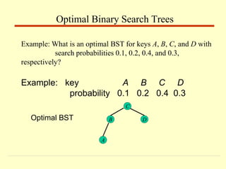
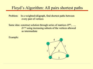
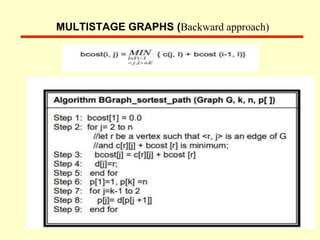
18. The left table is filled using the recurrence
C[i,j] = min {C[i,k-1] + C[k+1,j]} + ∑ ps , C[i,i] = pi
i ≤ k ≤ j s = i
The right saves the tree roots, which are the k’s that give the
minima
Example: key A B C D
probability 0.1 0.2 0.4 0.3
j
0 1 2 3 4
1 0 .1 .4 1.1 1.7
2 0 .2 .8 1.4
3 0 .4 1.0
4 0 .3
5 0
0 1 2 3 4
1 1 2 3 3
2 2 3 3
3 3 3
4 4
5
B
A
C
D

19. Contents

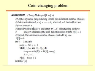
20. Time efficiency: Θ(n3) but can be reduced to Θ(n2) by taking
advantage of monotonicity of entries in the
root table, i.e., R[i,j] is always in the range
between R[i,j-1] and R[i+1,j]
Space efficiency: Θ(n2)
Method can be expanded to include unsuccessful searches
Analysis DP for Optimal BST Problem

21. Problem: In a weighted (di)graph, find shortest paths between
every pair of vertices
Same idea: construct solution through series of matrices D(0), …,
D (n) using increasing subsets of the vertices allowed
as intermediate
Example:
Floyd’s Algorithm: All pairs shortest paths
3
4
2
1
4
1
6
1
5
3

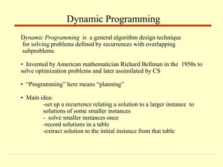
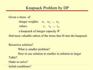
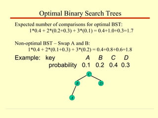
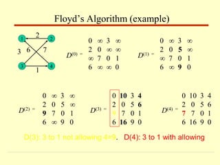
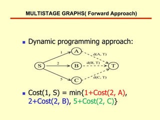
23. On the k-th iteration, the algorithm determines shortest paths
between every pair of vertices i, j that use only vertices among
1,…,k as intermediate
D(k)[i,j] = min {D(k-1)[i,j], D(k-1)[i,k] + D(k-1)[k,j]}
Floyd’s Algorithm (matrix generation)

24. Floyd’s Algorithm (example)
0 ∞ 3 ∞
2 0 ∞ ∞
∞ 7 0 1
6 ∞ ∞ 0
D(0) =
0 ∞ 3 ∞
2 0 5 ∞
∞ 7 0 1
6 ∞ 9 0
D(1) =
0 ∞ 3 ∞
2 0 5 ∞
9 7 0 1
6 ∞ 9 0
D(2) =
0 10 3 4
2 0 5 6
9 7 0 1
6 16 9 0
D(3) =
0 10 3 4
2 0 5 6
7 7 0 1
6 16 9 0
D(4) =
3
1
3
2
6 7
4
1 2

25. 3
1
3
2
6 7
4
1 2
0 ∞ 3 ∞
2 0 ∞ ∞
∞ 7 0 1
6 ∞ ∞ 0
D(0) =
1 2 4
3
1
2
3
4
D(1) =
1 2 4
3
1
2
3
4
D(2) =
1 2 4
3
1
2
3
4
0 10 3 4
2 0 5 6
9 7 0 1
6 16 9 0
D(3) =

26. Floyd’s Algorithm (pseudocode and analysis)
Time efficiency: Θ(n3)
Space efficiency: Matrices can be written over their predecessors
Note: Shortest paths themselves can be found, too

27. MULTISTAGE GRAPHS
• A multistage graph G = (V, E)is a directed graph in which
the vertices are partitioned into k ≥ 2 disjoint sets Vi, 1 ≤ i ≤
k.
• If <u,v> is an edge in E, then u∈ Vi and v∈ Vi+1 for some i,
1≤i ≤ k. The set V1 and Vk are such that |V1| = |Vk| = 1.
• Let s and t respectively, be the vertices in V1 and Vk
• The multistage graph problem is to find a minimum
costpath from s to t.

28. MULTISTAGE GRAPHS

31. MULTISTAGE GRAPHS ( Forward Approach)

32. MULTISTAGE GRAPHS (Backward approach)

33. MULTISTAGE GRAPHS( Forward Approach)
 Dynamic programming approach:
 Cost(1, S) = min{1+Cost(2, A),
2+Cost(2, B), 5+Cost(2, C)}
S T
2
B
A
C
1
5
d(C, T)
d(B, T)
d(A, T)

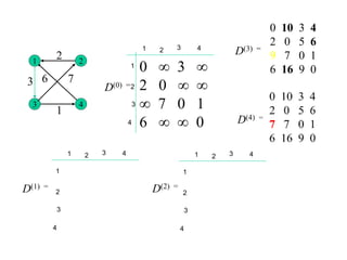
34. TRAVELLING SALESMAN PROBLEM
1 2 3 4
1 0 10 15 20
2 5 0 9 10
3 6 13 0 12
4 8 8 9 0
Cost( i, s)=min{Cost(j, s-(j))+d[ i, j]}

35. S = Φ
Cost(2,Φ,1)=d(2,1)=5
Cost(3,Φ,1)=d(3,1)=6
Cost(4,Φ,1)=d(4,1)=8
S = 1
Cost(2,{3},1)=d[2,3]+Cost(3,Φ,1)=9+6=15
Cost(2,{4},1)=d[2,4]+Cost(4,Φ,1)=10+8=18
Cost(3,{2},1)=d[3,2]+Cost(2,Φ,1)=13+5=18
Cost(3,{4},1)=d[3,4]+Cost(4,Φ,1)=12+8=20
Cost(4,{3},1)=d[4,3]+Cost(3,Φ,1)=9+6=15
Cost(4,{2},1)=d[4,2]+Cost(2,Φ,1)=8+5=13
S = 2
Cost(2,{3,4},1)=min{d[2,3]+Cost(3,{4},1),
d[2,4]+Cost(4,{3},1)}
= min {9+20,10+15} = min{29,25} = 25

36. Cost(3,{2,4},1)=min{d[3,2]+Cost(2,{4},1),
d[3,4]+Cost(4,{2},1)}
=min {13+18,12+13} = min {31, 25} = 25
Cost(4,{2,3},1)=min{d[4,2]+Cost(2,{3},1),
d[4,3]+Cost(3,{2},1)}
=min {8+15,9+18} = min {23,27} =23
S = 3
Cost(1,{2,3,4},1)=min{ d[1,2]+Cost(2,{3,4},1),
d[1,3]+Cost(3,{2,4},1), d[1,4]+cost(4,{2,3},1)}
=min{10+25, 15+25, 20+23} =
min{35,40,43}=35