SlideShare a Scribd company logo
1 of 41
Dynamic Programming
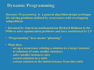
Dynamic Programming is a general algorithm design technique
for solving problems defined by recurrences with overlapping
subproblems
• Invented by American mathematician Richard Bellman in the
1950s to solve optimization problems and later assimilated by CS
• “Programming” here means “planning”
• Main idea:
- set up a recurrence relating a solution to a larger instance
to solutions of some smaller instances
- solve smaller instances once
- record solutions in a table
- extract solution to the initial instance from that table
Example 1: Fibonacci numbers
• Recall definition of Fibonacci numbers:
F(n) = F(n-1) + F(n-2)
F(0) = 0
F(1) = 1
• Computing the nth Fibonacci number recursively (top-down):
F(n)
F(n-1) + F(n-2)
F(n-2) + F(n-3) F(n-3) + F(n-4)
...
Example 1: Fibonacci numbers (cont.)
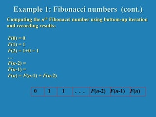
Computing the nth Fibonacci number using bottom-up iteration
and recording results:
F(0) = 0
F(1) = 1
F(2) = 1+0 = 1
…
F(n-2) =
F(n-1) =
F(n) = F(n-1) + F(n-2)
0 1 1 . . . F(n-2) F(n-1) F(n)
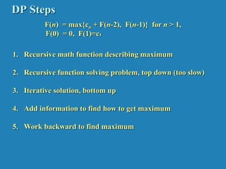
DP Steps
F(n) = max{cn + F(n-2), F(n-1)} for n > 1,
F(0) = 0, F(1)=c₁
1. Recursive math function describing maximum
2. Recursive function solving problem, top down (too slow)
3. Iterative solution, bottom up
4. Add information to find how to get maximum
5. Work backward to find maximum
Other examples of DP algorithms
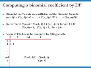
• Computing a binomial coefficient
•General case of the change making problem
• Some difficult discrete optimization problems:
- knapsack
- traveling salesman
• Constructing an optimal binary search tree
• Warshall’s algorithm for transitive closure
•Floyd’s algorithm for all-pairs shortest paths
Warshall’s Algorithm: Transitive Closure
• Computes the transitive closure of a relation
• Alternatively: existence of all nontrivial paths in a digraph
• Example of transitive closure:
3
4
2
1
0 0 1 0
1 0 0 1
0 0 0 0
0 1 0 0
0 0 1 0
1 1 1 1
0 0 0 0
1 1 1 1
3
4
2
1
Warshall’s Algorithm (recurrence)
On the k-th iteration, the algorithm determines for every pair of
vertices i, j if a path exists from i and j with just vertices 1,…,k
allowed as intermediate
R(k-1)[i,j] (path using just 1 ,…,k-1)
R(k)[i,j] = or
R(k-1)[i,k] and R(k-1)[k,j] (path from i to k
and from k to i
using just 1 ,…,k-1)
i
j
k
{
Warshall’s Algorithm (matrix generation)
Recurrence relating elements R(k) to elements of R(k-1) is:
R(k)[i,j] = R(k-1)[i,j] or (R(k-1)[i,k] and R(k-1)[k,j])
It implies the following rules for generating R(k) from R(k-1):
Rule 1 If an element in row i and column j is 1 in R(k-1),
it remains 1 in R(k)
Rule 2 If an element in row i and column j is 0 in R(k-1),
it has to be changed to 1 in R(k) if and only if
the element in its row i and column k and the element
in its column j and row k are both 1’s in R(k-1)
Warshall’s Algorithm
Constructs transitive closure T as the last matrix in the sequence
of n-by-n matrices R(0), … , R(k), … , R(n) where
R(k)[i,j] = 1 iff there is nontrivial path from i to j with only first k
vertices allowed as intermediate
Note that R(0) = A (adjacency matrix), R(n) = T (transitive closure)
3
4
2
1
3
4
2
1
3
4
2
1
3
4
2
1
R(0)
0 0 1 0
1 0 0 1
0 0 0 0
0 1 0 0
R(1)
0 0 1 0
1 0 1 1
0 0 0 0
0 1 0 0
R(2)
0 0 1 0
1 0 1 1
0 0 0 0
1 1 1 1
R(3)
0 0 1 0
1 0 1 1
0 0 0 0
1 1 1 1
R(4)
0 0 1 0
1 1 1 1
0 0 0 0
1 1 1 1
3
4
2
1
Warshall’s Algorithm (example)
3
4
2
1 0 0 1 0
1 0 0 1
0 0 0 0
0 1 0 0
R(0) =
0 0 1 0
1 0 1 1
0 0 0 0
0 1 0 0
R(1) =
0 0 1 0
1 0 1 1
0 0 0 0
1 1 1 1
R(2) =
0 0 1 0
1 0 1 1
0 0 0 0
1 1 1 1
R(3) =
0 0 1 0
1 1 1 1
0 0 0 0
1 1 1 1
R(4) =
Warshall’s Algorithm (pseudocode and analysis)
Time efficiency: Θ(n3)
Space efficiency: Matrices can be written over their predecessors
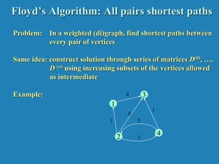
Floyd’s Algorithm: All pairs shortest paths
Problem: In a weighted (di)graph, find shortest paths between
every pair of vertices
Same idea: construct solution through series of matrices D(0), …,
D (n) using increasing subsets of the vertices allowed
as intermediate
Example: 3
4
2
1
4
1
6
1
5
3
Floyd’s Algorithm (matrix generation)
On the k-th iteration, the algorithm determines shortest paths
between every pair of vertices i, j that use only vertices among
1,…,k as intermediate
D(k)[i,j] = min {D(k-1)[i,j], D(k-1)[i,k] + D(k-1)[k,j]}
i
j
k
D(k-1)[i,j]
D(k-1)[i,k]
D(k-1)[k,j]
Floyd’s Algorithm (example)
0 ∞ 3 ∞
2 0 ∞ ∞
∞ 7 0 1
6 ∞ ∞ 0
D(0) =
0 ∞ 3 ∞
2 0 5 ∞
∞ 7 0 1
6 ∞ 9 0
D(1) =
0 ∞ 3 ∞
2 0 5 ∞
9 7 0 1
6 ∞ 9 0
D(2) =
0 10 3 4
2 0 5 6
9 7 0 1
6 16 9 0
D(3) =
0 10 3 4
2 0 5 6
7 7 0 1
6 16 9 0
D(4) =
3
1
3
2
6 7
4
1 2
D(3): 3 to 1 not allowing 4=9. D(4): 3 to 1 with allowing 4=7
Floyd’s Algorithm (pseudocode and analysis)
Time efficiency: Θ(n3)
Space efficiency: Matrices can be written over their predecessors
Note: Shortest paths themselves can be found, too (Problem 10)
Assignment
Knapsack Problem by DP
Given n items of
integer weights: w1 w2 … wn
values: v1 v2 … vn
a knapsack of integer capacity W
find most valuable subset of the items that fit into the knapsack
Consider instance defined by first i items and capacity j (j  W).
Let V[i,j] be optimal value of such instance. Then
max {V[i-1,j], vi + V[i-1,j- wi]} if j- wi  0
V[i,j] =
V[i-1,j] if j- wi < 0
Initial conditions: V[0,j] = 0 and V[i,0] = 0
• Let F(i, j) be the value of an optimal solution to
this instance, i.e., the value of the most valuable
subset of the first i items that fit into the knapsack
of capacity j.
• We can divide all the subsets of the first i items
that fit the knapsack of capacity j into two
categories: those that do not include the ith item
and those that do.
• Our goal is to find F (n, W),the maximal value of
a subset of then given items that fit into the
knapsack of capacity W, and an optimal subset
itself.
Knapsack Problem by DP
Table for solving the knapsack problem by dynamic
programming
Recurrence relation for the knapsack problem by dynamic
programming
Knapsack Problem by DP (example)
Example: Knapsack of capacity W = 5
item weight value
1 2 $12
2 1 $10
3 3 $20
4 2 $15 capacity j
0 1 2 3 4 5
0 0 0 0 0 0 0
w1 = 2, v1= 12 1 0 0
w2 = 1, v2= 10 2
w3 = 3, v3= 20 3
w4 = 2, v4= 15 4 ?
Knapsack Problem by DP (example)
Example: Knapsack of capacity W = 5
item weight value
1 2 $12
2 1 $10
3 3 $20
4 2 $15 capacity j
0 1 2 3 4 5
0 0 0 0 0 0 0
w1 = 2, v1= 12 1 0 0 12 12 12 12
w2 = 1, v2= 10 2 0 10 12 22 22 22
w3 = 3, v3= 20 3 0 10 12 22 30 32
w4 = 2, v4= 15 4 0 10 15 25 30 37
Knapsack Problem by DP (example)
V[i,j]= max(v[i-1, j] , vi + v[i-1, j-wi] if j-wi >=0
v[i-1, j] if j-wi < 0
v[1,1] = 1-2= -1 j-wi<0 = v[0,1]=0
v[1,2]=max(0,12+0)=12
v[2,3]=max(12,10+12)=22
v[3,5]=max(22,20+12)=32
capacity j
0 1 2 3 4 5
0 0 0 0 0 0 0
w1 = 2, v1= 12 1 0 0 12 12 12 12
w2 = 1, v2= 10 2 0 10 12 22 22 22
w3 = 3, v3= 20 3 0 10 12 22 30 32
w4 = 2, v = 15 4 0 10 15 25 30 37
Knapsack Problem by DP (example)
V[i,j]= max(v[i-1, j] , vi + v[i-1, j-wi] if j-wi >=0
v[i-1, j] if j-wi < 0
v[1,1] = 1-2= -1 j-wi<0 = v[0,1]=0
v[1,2]=max(0,12+0)=12 v[4,5]= max(32, 15+22) =37
v[2,3]=max(12,10+12)=22
v[3,5]=max(22,20+12)=32
capacity j
0 1 2 3 4 5
0 0 0 0 0 0 0
w1 = 2, v1= 12 1 0 0 12 12 12 12
w2 = 1, v2= 10 2 0 10 12 22 22 22
w3 = 3, v3= 20 3 0 10 12 22 30 32
w4 = 2, v4= 15 4 0 10 15 25 30 37
To know which objects are placed, v[objects, capacity]
If v[4,5] != v[3,5], 4th object is placed else it is not placed
37 != 32 therefore 4th object is placed
Decrease the capacity by the weight of the object
v[3, 5-2]= v[3,3] = v[2,3] , object 3 not placed
v[2,3]!= v[1,3]] 2nd object is placed
v[1, 3-1] = v[1,2] != v[0,2], 1st object is placed
capacity j
0 1 2 3 4 5
0 0 0 0 0 0 0
w1 = 2, v1= 12 1 0 0 12 12 12 12
w2 = 1, v2= 10 2 0 10 12 22 22 22
w3 = 3, v3= 20 3 0 10 12 22 30 32
w4 = 2, v4= 15 4 0 10 15 25 30 37
Optimal Binary Search Trees
Problem: Given n keys a1 < …< an and probabilities p1 ≤ … ≤ pn
searching for them, find a BST with a minimum
average number of comparisons in successful search.
Since total number of BSTs with n nodes is given by
C(2n,n)/(n+1), which grows exponentially, brute force is hopeless.
Example: What is an optimal BST for keys A, B, C, and D with
search probabilities 0.1, 0.2, 0.4, and 0.3, respectively?
What smaller problems could we use?
Let’s first look at an example.
Example: key A B C D
probability 0.1 0.2 0.4 0.3
Expected number of comparisons?
optimal BST
B
A
C
D
Example: key A B C D
probability 0.1 0.2 0.4 0.3
Expected number of comparisons for optimal BST:
1*0.4 + 2*(0.2+0.3) + 3*(0.1) = 0.4+1.0+0.3=1.7
Non-optimal BST – Swap A and B:
1*0.4 + 2*(0.1+0.3) + 3*(0.2) = 0.4+0.8+0.6=1.8
optimal BST
B
A
C
D
Example: key A B C D
probability 0.1 0.2 0.4 0.3
Expected number of comparisons for optimal BST:
1*0.4 + 2*(0.2+0.3) + 3*(0.1) = 0.4+1.0+0.3=1.7
Can factor out cost of visiting each node once:
1*0.4 + 2*(0.2+0.3) + 3*(0.1) = 0*.4+1*.5+2*.1 + 1*(.4+.5+.1)
Moving subtree up or down changes total by weight of subtree
- BA at level 1/2 has cost 1*.2 + 2*.1 = .4 =
- BA at level 2/3 has cost 2*.2 + 3*.1 = .7 = .4 + (.2 + .1)
- BA at level 3/4 has cost ???
optimal BST
B
A
C
D
Example: key A B C D
probability 0.1 0.2 0.4 0.3
Expected number of comparisons for optimal BST:
1*0.4 + 2*(0.2+0.3) + 3*(0.1) = 0.4+1.0+0.3=1.7
Can factor out cost of visiting each node once:
1*0.4 + 2*(0.2+0.3) + 3*(0.1) = 0*.4+1*.5+2*.1 + 1*(.4+.5+.1)
Moving subtree up or down changes total by weight of subtree
- BA at level 1/2 has cost 1*.2 + 2*.1 = 0.4 =
- BA at level 2/3 has cost 2*.2 + 3*.1 = 0.7 = .4 + (.2 + .1)
- BA at level 3/4 has cost 3*.2 + 4*.1 = 1.0 = .4 + (.2 + .1)
optimal BST
B
A
C
D
Optimal Binary Search Trees
Problem: Given n keys a1 < …< an and probabilities p1 ≤ … ≤ pn
searching for them, find a BST with a minimum
average number of comparisons in successful search.
What smaller problems could we use?
Optimal Binary Search Trees
Problem: Given n keys a1 < …< an and probabilities p1 ≤ … ≤ pn
searching for them, find a BST with a minimum
average number of comparisons in successful search.
What smaller problems could we use?
What if we let each element be the root?
What is needed then?
DP for Optimal BST Problem
Let T[i,j] be optimal BST for keys ai < …< aj , C[i,j] be minimum
average number of comparisons made in T[i,j], for 1 ≤ i ≤ j ≤ n.
Consider optimal BST among all BSTs with some ak (i ≤ k ≤ j )
as their root; T[i,j] is the best among them.
a
Optimal
BST for
a , ..., a
Optimal
BST for
a , ..., a
i
k
k-1 k+1 j
C[i,j] =
min {pk · 1 +
∑ ps · (level as in T[i,k-1] +1) +
∑ ps · (level as in T[k+1,j] +1)}
i ≤ k ≤ j
s = i
k-1
s =k+1
j
Min Num Comparisons
Best Tree
DP for Optimal BST Problem (cont.)
After simplifications, we obtain the recurrence for C[i,j]:
C[i,j] = min {C[i,k-1] + C[k+1,j]} + ∑ ps for 1 ≤ i ≤ j ≤ n
C[i,i] = pi for 1 ≤ i ≤ j ≤ n
What table elements are involved?
s = i
j
i ≤ k ≤ j
goal
0
0
C[i,j]
0
1
n+1
0 1 n
p 1
p2
n
p
i
j
DP for Optimal BST Problem (cont.)
After simplifications, we obtain the recurrence for C[i,j]:
C[i,j] = min {C[i,k-1] + C[k+1,j]} + ∑ ps for 1 ≤ i ≤ j ≤ n
C[i,i] = pi for 1 ≤ i ≤ j ≤ n
s = i
j
i ≤ k ≤ j
Example: key A B C D
probability 0.1 0.2 0.4 0.3
The left table is filled using the recurrence
C[i,j] = min {C[i,k-1] + C[k+1,j]} + ∑ ps , C[i,i] = pi
The right saves the tree roots, which are the k’s that give the minima
0 1 2 3 4
1 0 .1 .4 1.1 1.7
2 0 .2 .8 1.4
3 0 .4 1.0
4 0 .3
5 0
0 1 2 3 4
1 1 2 3 3
2 2 3 3
3 3 3
4 4
5
i ≤ k ≤ j s = i
j
optimal BST
B
A
C
D
i
j i
j
Tables filled diagonal by diagonal (remember what C[i,j] is).
Optimal Binary Search Trees
Analysis DP for Optimal BST Problem
Time efficiency: Θ(n3) but can be reduced to Θ(n2) by taking
advantage of monotonicity of entries in the
root table, i.e., R[i,j] is always in the range
between R[i,j-1] and R[i+1,j]
Space efficiency: Θ(n2)
Method can be expanded to include unsuccessful searches

More Related Content

Similar to Dynamic Programming for 4th sem cse students

Binomial Theorem
Binomial TheoremBinomial Theorem
Binomial Theoremitutor
 
Additional mathematics
Additional mathematicsAdditional mathematics
Additional mathematicsgeraldsiew
 
01 knapsack using backtracking
01 knapsack using backtracking01 knapsack using backtracking
01 knapsack using backtrackingmandlapure
 
Integration techniques
Integration techniquesIntegration techniques
Integration techniquesKrishna Gali
 
Recursion - Computer Algorithms
Recursion - Computer AlgorithmsRecursion - Computer Algorithms
Recursion - Computer AlgorithmsAlaa Al-Makhzoomy
 
Random Matrix Theory and Machine Learning - Part 3
Random Matrix Theory and Machine Learning - Part 3Random Matrix Theory and Machine Learning - Part 3
Random Matrix Theory and Machine Learning - Part 3Fabian Pedregosa
 
Divide-and-Conquer & Dynamic ProgrammingDivide-and-Conqu.docx
Divide-and-Conquer & Dynamic ProgrammingDivide-and-Conqu.docxDivide-and-Conquer & Dynamic ProgrammingDivide-and-Conqu.docx
Divide-and-Conquer & Dynamic ProgrammingDivide-and-Conqu.docxjacksnathalie
 
Laplace equation
Laplace equationLaplace equation
Laplace equationalexkhan129
 
Analysis Of Algorithms Ii
Analysis Of Algorithms IiAnalysis Of Algorithms Ii
Analysis Of Algorithms IiSri Prasanna
 
Integer_Functions .pdf
Integer_Functions .pdfInteger_Functions .pdf
Integer_Functions .pdfJainggaPotla
 
Succesive differntiation
Succesive differntiationSuccesive differntiation
Succesive differntiationJaydevVadachhak
 
Review for the Third Midterm of Math 150 B 11242014Probl.docx
Review for the Third Midterm of Math 150 B 11242014Probl.docxReview for the Third Midterm of Math 150 B 11242014Probl.docx
Review for the Third Midterm of Math 150 B 11242014Probl.docxjoellemurphey
 
Solving the energy problem of helium final report
Solving the energy problem of helium final reportSolving the energy problem of helium final report
Solving the energy problem of helium final reportJamesMa54
 
Crib Sheet AP Calculus AB and BC exams
Crib Sheet AP Calculus AB and BC examsCrib Sheet AP Calculus AB and BC exams
Crib Sheet AP Calculus AB and BC examsA Jorge Garcia
 

Similar to Dynamic Programming for 4th sem cse students (20)

Binomial Theorem
Binomial TheoremBinomial Theorem
Binomial Theorem
 
Randomized algorithms ver 1.0
Randomized algorithms ver 1.0Randomized algorithms ver 1.0
Randomized algorithms ver 1.0
 
Aieee maths-2003
Aieee maths-2003Aieee maths-2003
Aieee maths-2003
 
Additional mathematics
Additional mathematicsAdditional mathematics
Additional mathematics
 
Vector space
Vector spaceVector space
Vector space
 
01 knapsack using backtracking
01 knapsack using backtracking01 knapsack using backtracking
01 knapsack using backtracking
 
Integration techniques
Integration techniquesIntegration techniques
Integration techniques
 
Recursion - Computer Algorithms
Recursion - Computer AlgorithmsRecursion - Computer Algorithms
Recursion - Computer Algorithms
 
Random Matrix Theory and Machine Learning - Part 3
Random Matrix Theory and Machine Learning - Part 3Random Matrix Theory and Machine Learning - Part 3
Random Matrix Theory and Machine Learning - Part 3
 
Divide-and-Conquer & Dynamic ProgrammingDivide-and-Conqu.docx
Divide-and-Conquer & Dynamic ProgrammingDivide-and-Conqu.docxDivide-and-Conquer & Dynamic ProgrammingDivide-and-Conqu.docx
Divide-and-Conquer & Dynamic ProgrammingDivide-and-Conqu.docx
 
Laplace equation
Laplace equationLaplace equation
Laplace equation
 
Analysis Of Algorithms Ii
Analysis Of Algorithms IiAnalysis Of Algorithms Ii
Analysis Of Algorithms Ii
 
Integer_Functions .pdf
Integer_Functions .pdfInteger_Functions .pdf
Integer_Functions .pdf
 
ch3.ppt
ch3.pptch3.ppt
ch3.ppt
 
Succesive differntiation
Succesive differntiationSuccesive differntiation
Succesive differntiation
 
Review for the Third Midterm of Math 150 B 11242014Probl.docx
Review for the Third Midterm of Math 150 B 11242014Probl.docxReview for the Third Midterm of Math 150 B 11242014Probl.docx
Review for the Third Midterm of Math 150 B 11242014Probl.docx
 
Lecture5
Lecture5Lecture5
Lecture5
 
Solving the energy problem of helium final report
Solving the energy problem of helium final reportSolving the energy problem of helium final report
Solving the energy problem of helium final report
 
Crib Sheet AP Calculus AB and BC exams
Crib Sheet AP Calculus AB and BC examsCrib Sheet AP Calculus AB and BC exams
Crib Sheet AP Calculus AB and BC exams
 
Ch4
Ch4Ch4
Ch4
 

Recently uploaded

internship ppt on smartinternz platform as salesforce developer
internship ppt on smartinternz platform as salesforce developerinternship ppt on smartinternz platform as salesforce developer
internship ppt on smartinternz platform as salesforce developerunnathinaik
 
Paris 2024 Olympic Geographies - an activity
Paris 2024 Olympic Geographies - an activityParis 2024 Olympic Geographies - an activity
Paris 2024 Olympic Geographies - an activityGeoBlogs
 
Sanyam Choudhary Chemistry practical.pdf
Sanyam Choudhary Chemistry practical.pdfSanyam Choudhary Chemistry practical.pdf
Sanyam Choudhary Chemistry practical.pdfsanyamsingh5019
 
BASLIQ CURRENT LOOKBOOK LOOKBOOK(1) (1).pdf
BASLIQ CURRENT LOOKBOOK  LOOKBOOK(1) (1).pdfBASLIQ CURRENT LOOKBOOK  LOOKBOOK(1) (1).pdf
BASLIQ CURRENT LOOKBOOK LOOKBOOK(1) (1).pdfSoniaTolstoy
 
Painted Grey Ware.pptx, PGW Culture of India
Painted Grey Ware.pptx, PGW Culture of IndiaPainted Grey Ware.pptx, PGW Culture of India
Painted Grey Ware.pptx, PGW Culture of IndiaVirag Sontakke
 
“Oh GOSH! Reflecting on Hackteria's Collaborative Practices in a Global Do-It...
“Oh GOSH! Reflecting on Hackteria's Collaborative Practices in a Global Do-It...“Oh GOSH! Reflecting on Hackteria's Collaborative Practices in a Global Do-It...
“Oh GOSH! Reflecting on Hackteria's Collaborative Practices in a Global Do-It...Marc Dusseiller Dusjagr
 
18-04-UA_REPORT_MEDIALITERAСY_INDEX-DM_23-1-final-eng.pdf
18-04-UA_REPORT_MEDIALITERAСY_INDEX-DM_23-1-final-eng.pdf18-04-UA_REPORT_MEDIALITERAСY_INDEX-DM_23-1-final-eng.pdf
18-04-UA_REPORT_MEDIALITERAСY_INDEX-DM_23-1-final-eng.pdfssuser54595a
 
Organic Name Reactions for the students and aspirants of Chemistry12th.pptx
Organic Name Reactions  for the students and aspirants of Chemistry12th.pptxOrganic Name Reactions  for the students and aspirants of Chemistry12th.pptx
Organic Name Reactions for the students and aspirants of Chemistry12th.pptxVS Mahajan Coaching Centre
 
Hybridoma Technology ( Production , Purification , and Application )
Hybridoma Technology  ( Production , Purification , and Application  ) Hybridoma Technology  ( Production , Purification , and Application  )
Hybridoma Technology ( Production , Purification , and Application ) Sakshi Ghasle
 
ENGLISH5 QUARTER4 MODULE1 WEEK1-3 How Visual and Multimedia Elements.pptx
ENGLISH5 QUARTER4 MODULE1 WEEK1-3 How Visual and Multimedia Elements.pptxENGLISH5 QUARTER4 MODULE1 WEEK1-3 How Visual and Multimedia Elements.pptx
ENGLISH5 QUARTER4 MODULE1 WEEK1-3 How Visual and Multimedia Elements.pptxAnaBeatriceAblay2
 
SOCIAL AND HISTORICAL CONTEXT - LFTVD.pptx
SOCIAL AND HISTORICAL CONTEXT - LFTVD.pptxSOCIAL AND HISTORICAL CONTEXT - LFTVD.pptx
SOCIAL AND HISTORICAL CONTEXT - LFTVD.pptxiammrhaywood
 
Software Engineering Methodologies (overview)
Software Engineering Methodologies (overview)Software Engineering Methodologies (overview)
Software Engineering Methodologies (overview)eniolaolutunde
 
Employee wellbeing at the workplace.pptx
Employee wellbeing at the workplace.pptxEmployee wellbeing at the workplace.pptx
Employee wellbeing at the workplace.pptxNirmalaLoungPoorunde1
 
Presiding Officer Training module 2024 lok sabha elections
Presiding Officer Training module 2024 lok sabha electionsPresiding Officer Training module 2024 lok sabha elections
Presiding Officer Training module 2024 lok sabha electionsanshu789521
 
Computed Fields and api Depends in the Odoo 17
Computed Fields and api Depends in the Odoo 17Computed Fields and api Depends in the Odoo 17
Computed Fields and api Depends in the Odoo 17Celine George
 
Science 7 - LAND and SEA BREEZE and its Characteristics
Science 7 - LAND and SEA BREEZE and its CharacteristicsScience 7 - LAND and SEA BREEZE and its Characteristics
Science 7 - LAND and SEA BREEZE and its CharacteristicsKarinaGenton
 
Solving Puzzles Benefits Everyone (English).pptx
Solving Puzzles Benefits Everyone (English).pptxSolving Puzzles Benefits Everyone (English).pptx
Solving Puzzles Benefits Everyone (English).pptxOH TEIK BIN
 

Recently uploaded (20)

internship ppt on smartinternz platform as salesforce developer
internship ppt on smartinternz platform as salesforce developerinternship ppt on smartinternz platform as salesforce developer
internship ppt on smartinternz platform as salesforce developer
 
Paris 2024 Olympic Geographies - an activity
Paris 2024 Olympic Geographies - an activityParis 2024 Olympic Geographies - an activity
Paris 2024 Olympic Geographies - an activity
 
Sanyam Choudhary Chemistry practical.pdf
Sanyam Choudhary Chemistry practical.pdfSanyam Choudhary Chemistry practical.pdf
Sanyam Choudhary Chemistry practical.pdf
 
BASLIQ CURRENT LOOKBOOK LOOKBOOK(1) (1).pdf
BASLIQ CURRENT LOOKBOOK  LOOKBOOK(1) (1).pdfBASLIQ CURRENT LOOKBOOK  LOOKBOOK(1) (1).pdf
BASLIQ CURRENT LOOKBOOK LOOKBOOK(1) (1).pdf
 
Painted Grey Ware.pptx, PGW Culture of India
Painted Grey Ware.pptx, PGW Culture of IndiaPainted Grey Ware.pptx, PGW Culture of India
Painted Grey Ware.pptx, PGW Culture of India
 
“Oh GOSH! Reflecting on Hackteria's Collaborative Practices in a Global Do-It...
“Oh GOSH! Reflecting on Hackteria's Collaborative Practices in a Global Do-It...“Oh GOSH! Reflecting on Hackteria's Collaborative Practices in a Global Do-It...
“Oh GOSH! Reflecting on Hackteria's Collaborative Practices in a Global Do-It...
 
18-04-UA_REPORT_MEDIALITERAСY_INDEX-DM_23-1-final-eng.pdf
18-04-UA_REPORT_MEDIALITERAСY_INDEX-DM_23-1-final-eng.pdf18-04-UA_REPORT_MEDIALITERAСY_INDEX-DM_23-1-final-eng.pdf
18-04-UA_REPORT_MEDIALITERAСY_INDEX-DM_23-1-final-eng.pdf
 
Model Call Girl in Bikash Puri Delhi reach out to us at 🔝9953056974🔝
Model Call Girl in Bikash Puri  Delhi reach out to us at 🔝9953056974🔝Model Call Girl in Bikash Puri  Delhi reach out to us at 🔝9953056974🔝
Model Call Girl in Bikash Puri Delhi reach out to us at 🔝9953056974🔝
 
Organic Name Reactions for the students and aspirants of Chemistry12th.pptx
Organic Name Reactions  for the students and aspirants of Chemistry12th.pptxOrganic Name Reactions  for the students and aspirants of Chemistry12th.pptx
Organic Name Reactions for the students and aspirants of Chemistry12th.pptx
 
Hybridoma Technology ( Production , Purification , and Application )
Hybridoma Technology  ( Production , Purification , and Application  ) Hybridoma Technology  ( Production , Purification , and Application  )
Hybridoma Technology ( Production , Purification , and Application )
 
ENGLISH5 QUARTER4 MODULE1 WEEK1-3 How Visual and Multimedia Elements.pptx
ENGLISH5 QUARTER4 MODULE1 WEEK1-3 How Visual and Multimedia Elements.pptxENGLISH5 QUARTER4 MODULE1 WEEK1-3 How Visual and Multimedia Elements.pptx
ENGLISH5 QUARTER4 MODULE1 WEEK1-3 How Visual and Multimedia Elements.pptx
 
SOCIAL AND HISTORICAL CONTEXT - LFTVD.pptx
SOCIAL AND HISTORICAL CONTEXT - LFTVD.pptxSOCIAL AND HISTORICAL CONTEXT - LFTVD.pptx
SOCIAL AND HISTORICAL CONTEXT - LFTVD.pptx
 
Software Engineering Methodologies (overview)
Software Engineering Methodologies (overview)Software Engineering Methodologies (overview)
Software Engineering Methodologies (overview)
 
Employee wellbeing at the workplace.pptx
Employee wellbeing at the workplace.pptxEmployee wellbeing at the workplace.pptx
Employee wellbeing at the workplace.pptx
 
Presiding Officer Training module 2024 lok sabha elections
Presiding Officer Training module 2024 lok sabha electionsPresiding Officer Training module 2024 lok sabha elections
Presiding Officer Training module 2024 lok sabha elections
 
Staff of Color (SOC) Retention Efforts DDSD
Staff of Color (SOC) Retention Efforts DDSDStaff of Color (SOC) Retention Efforts DDSD
Staff of Color (SOC) Retention Efforts DDSD
 
Computed Fields and api Depends in the Odoo 17
Computed Fields and api Depends in the Odoo 17Computed Fields and api Depends in the Odoo 17
Computed Fields and api Depends in the Odoo 17
 
Science 7 - LAND and SEA BREEZE and its Characteristics
Science 7 - LAND and SEA BREEZE and its CharacteristicsScience 7 - LAND and SEA BREEZE and its Characteristics
Science 7 - LAND and SEA BREEZE and its Characteristics
 
Solving Puzzles Benefits Everyone (English).pptx
Solving Puzzles Benefits Everyone (English).pptxSolving Puzzles Benefits Everyone (English).pptx
Solving Puzzles Benefits Everyone (English).pptx
 
TataKelola dan KamSiber Kecerdasan Buatan v022.pdf
TataKelola dan KamSiber Kecerdasan Buatan v022.pdfTataKelola dan KamSiber Kecerdasan Buatan v022.pdf
TataKelola dan KamSiber Kecerdasan Buatan v022.pdf
 

Dynamic Programming for 4th sem cse students

  • 1. Dynamic Programming Dynamic Programming is a general algorithm design technique for solving problems defined by recurrences with overlapping subproblems • Invented by American mathematician Richard Bellman in the 1950s to solve optimization problems and later assimilated by CS • “Programming” here means “planning” • Main idea: - set up a recurrence relating a solution to a larger instance to solutions of some smaller instances - solve smaller instances once - record solutions in a table - extract solution to the initial instance from that table
  • 2. Example 1: Fibonacci numbers • Recall definition of Fibonacci numbers: F(n) = F(n-1) + F(n-2) F(0) = 0 F(1) = 1 • Computing the nth Fibonacci number recursively (top-down): F(n) F(n-1) + F(n-2) F(n-2) + F(n-3) F(n-3) + F(n-4) ...
  • 3. Example 1: Fibonacci numbers (cont.) Computing the nth Fibonacci number using bottom-up iteration and recording results: F(0) = 0 F(1) = 1 F(2) = 1+0 = 1 … F(n-2) = F(n-1) = F(n) = F(n-1) + F(n-2) 0 1 1 . . . F(n-2) F(n-1) F(n)
  • 4. DP Steps F(n) = max{cn + F(n-2), F(n-1)} for n > 1, F(0) = 0, F(1)=c₁ 1. Recursive math function describing maximum 2. Recursive function solving problem, top down (too slow) 3. Iterative solution, bottom up 4. Add information to find how to get maximum 5. Work backward to find maximum
  • 5. Other examples of DP algorithms • Computing a binomial coefficient •General case of the change making problem • Some difficult discrete optimization problems: - knapsack - traveling salesman • Constructing an optimal binary search tree • Warshall’s algorithm for transitive closure •Floyd’s algorithm for all-pairs shortest paths
  • 6.
  • 7.
  • 8. Warshall’s Algorithm: Transitive Closure • Computes the transitive closure of a relation • Alternatively: existence of all nontrivial paths in a digraph • Example of transitive closure: 3 4 2 1 0 0 1 0 1 0 0 1 0 0 0 0 0 1 0 0 0 0 1 0 1 1 1 1 0 0 0 0 1 1 1 1 3 4 2 1
  • 9. Warshall’s Algorithm (recurrence) On the k-th iteration, the algorithm determines for every pair of vertices i, j if a path exists from i and j with just vertices 1,…,k allowed as intermediate R(k-1)[i,j] (path using just 1 ,…,k-1) R(k)[i,j] = or R(k-1)[i,k] and R(k-1)[k,j] (path from i to k and from k to i using just 1 ,…,k-1) i j k {
  • 10. Warshall’s Algorithm (matrix generation) Recurrence relating elements R(k) to elements of R(k-1) is: R(k)[i,j] = R(k-1)[i,j] or (R(k-1)[i,k] and R(k-1)[k,j]) It implies the following rules for generating R(k) from R(k-1): Rule 1 If an element in row i and column j is 1 in R(k-1), it remains 1 in R(k) Rule 2 If an element in row i and column j is 0 in R(k-1), it has to be changed to 1 in R(k) if and only if the element in its row i and column k and the element in its column j and row k are both 1’s in R(k-1)
  • 11. Warshall’s Algorithm Constructs transitive closure T as the last matrix in the sequence of n-by-n matrices R(0), … , R(k), … , R(n) where R(k)[i,j] = 1 iff there is nontrivial path from i to j with only first k vertices allowed as intermediate Note that R(0) = A (adjacency matrix), R(n) = T (transitive closure) 3 4 2 1 3 4 2 1 3 4 2 1 3 4 2 1 R(0) 0 0 1 0 1 0 0 1 0 0 0 0 0 1 0 0 R(1) 0 0 1 0 1 0 1 1 0 0 0 0 0 1 0 0 R(2) 0 0 1 0 1 0 1 1 0 0 0 0 1 1 1 1 R(3) 0 0 1 0 1 0 1 1 0 0 0 0 1 1 1 1 R(4) 0 0 1 0 1 1 1 1 0 0 0 0 1 1 1 1 3 4 2 1
  • 12. Warshall’s Algorithm (example) 3 4 2 1 0 0 1 0 1 0 0 1 0 0 0 0 0 1 0 0 R(0) = 0 0 1 0 1 0 1 1 0 0 0 0 0 1 0 0 R(1) = 0 0 1 0 1 0 1 1 0 0 0 0 1 1 1 1 R(2) = 0 0 1 0 1 0 1 1 0 0 0 0 1 1 1 1 R(3) = 0 0 1 0 1 1 1 1 0 0 0 0 1 1 1 1 R(4) =
  • 13.
  • 14. Warshall’s Algorithm (pseudocode and analysis) Time efficiency: Θ(n3) Space efficiency: Matrices can be written over their predecessors
  • 15. Floyd’s Algorithm: All pairs shortest paths Problem: In a weighted (di)graph, find shortest paths between every pair of vertices Same idea: construct solution through series of matrices D(0), …, D (n) using increasing subsets of the vertices allowed as intermediate Example: 3 4 2 1 4 1 6 1 5 3
  • 16. Floyd’s Algorithm (matrix generation) On the k-th iteration, the algorithm determines shortest paths between every pair of vertices i, j that use only vertices among 1,…,k as intermediate D(k)[i,j] = min {D(k-1)[i,j], D(k-1)[i,k] + D(k-1)[k,j]} i j k D(k-1)[i,j] D(k-1)[i,k] D(k-1)[k,j]
  • 17. Floyd’s Algorithm (example) 0 ∞ 3 ∞ 2 0 ∞ ∞ ∞ 7 0 1 6 ∞ ∞ 0 D(0) = 0 ∞ 3 ∞ 2 0 5 ∞ ∞ 7 0 1 6 ∞ 9 0 D(1) = 0 ∞ 3 ∞ 2 0 5 ∞ 9 7 0 1 6 ∞ 9 0 D(2) = 0 10 3 4 2 0 5 6 9 7 0 1 6 16 9 0 D(3) = 0 10 3 4 2 0 5 6 7 7 0 1 6 16 9 0 D(4) = 3 1 3 2 6 7 4 1 2 D(3): 3 to 1 not allowing 4=9. D(4): 3 to 1 with allowing 4=7
  • 18. Floyd’s Algorithm (pseudocode and analysis) Time efficiency: Θ(n3) Space efficiency: Matrices can be written over their predecessors Note: Shortest paths themselves can be found, too (Problem 10)
  • 19.
  • 21. Knapsack Problem by DP Given n items of integer weights: w1 w2 … wn values: v1 v2 … vn a knapsack of integer capacity W find most valuable subset of the items that fit into the knapsack Consider instance defined by first i items and capacity j (j  W). Let V[i,j] be optimal value of such instance. Then max {V[i-1,j], vi + V[i-1,j- wi]} if j- wi  0 V[i,j] = V[i-1,j] if j- wi < 0 Initial conditions: V[0,j] = 0 and V[i,0] = 0
  • 22. • Let F(i, j) be the value of an optimal solution to this instance, i.e., the value of the most valuable subset of the first i items that fit into the knapsack of capacity j. • We can divide all the subsets of the first i items that fit the knapsack of capacity j into two categories: those that do not include the ith item and those that do. • Our goal is to find F (n, W),the maximal value of a subset of then given items that fit into the knapsack of capacity W, and an optimal subset itself. Knapsack Problem by DP
  • 23. Table for solving the knapsack problem by dynamic programming Recurrence relation for the knapsack problem by dynamic programming
  • 24. Knapsack Problem by DP (example) Example: Knapsack of capacity W = 5 item weight value 1 2 $12 2 1 $10 3 3 $20 4 2 $15 capacity j 0 1 2 3 4 5 0 0 0 0 0 0 0 w1 = 2, v1= 12 1 0 0 w2 = 1, v2= 10 2 w3 = 3, v3= 20 3 w4 = 2, v4= 15 4 ?
  • 25. Knapsack Problem by DP (example) Example: Knapsack of capacity W = 5 item weight value 1 2 $12 2 1 $10 3 3 $20 4 2 $15 capacity j 0 1 2 3 4 5 0 0 0 0 0 0 0 w1 = 2, v1= 12 1 0 0 12 12 12 12 w2 = 1, v2= 10 2 0 10 12 22 22 22 w3 = 3, v3= 20 3 0 10 12 22 30 32 w4 = 2, v4= 15 4 0 10 15 25 30 37
  • 26. Knapsack Problem by DP (example) V[i,j]= max(v[i-1, j] , vi + v[i-1, j-wi] if j-wi >=0 v[i-1, j] if j-wi < 0 v[1,1] = 1-2= -1 j-wi<0 = v[0,1]=0 v[1,2]=max(0,12+0)=12 v[2,3]=max(12,10+12)=22 v[3,5]=max(22,20+12)=32 capacity j 0 1 2 3 4 5 0 0 0 0 0 0 0 w1 = 2, v1= 12 1 0 0 12 12 12 12 w2 = 1, v2= 10 2 0 10 12 22 22 22 w3 = 3, v3= 20 3 0 10 12 22 30 32 w4 = 2, v = 15 4 0 10 15 25 30 37
  • 27. Knapsack Problem by DP (example) V[i,j]= max(v[i-1, j] , vi + v[i-1, j-wi] if j-wi >=0 v[i-1, j] if j-wi < 0 v[1,1] = 1-2= -1 j-wi<0 = v[0,1]=0 v[1,2]=max(0,12+0)=12 v[4,5]= max(32, 15+22) =37 v[2,3]=max(12,10+12)=22 v[3,5]=max(22,20+12)=32 capacity j 0 1 2 3 4 5 0 0 0 0 0 0 0 w1 = 2, v1= 12 1 0 0 12 12 12 12 w2 = 1, v2= 10 2 0 10 12 22 22 22 w3 = 3, v3= 20 3 0 10 12 22 30 32 w4 = 2, v4= 15 4 0 10 15 25 30 37
  • 28. To know which objects are placed, v[objects, capacity] If v[4,5] != v[3,5], 4th object is placed else it is not placed 37 != 32 therefore 4th object is placed Decrease the capacity by the weight of the object v[3, 5-2]= v[3,3] = v[2,3] , object 3 not placed v[2,3]!= v[1,3]] 2nd object is placed v[1, 3-1] = v[1,2] != v[0,2], 1st object is placed capacity j 0 1 2 3 4 5 0 0 0 0 0 0 0 w1 = 2, v1= 12 1 0 0 12 12 12 12 w2 = 1, v2= 10 2 0 10 12 22 22 22 w3 = 3, v3= 20 3 0 10 12 22 30 32 w4 = 2, v4= 15 4 0 10 15 25 30 37
  • 29. Optimal Binary Search Trees Problem: Given n keys a1 < …< an and probabilities p1 ≤ … ≤ pn searching for them, find a BST with a minimum average number of comparisons in successful search. Since total number of BSTs with n nodes is given by C(2n,n)/(n+1), which grows exponentially, brute force is hopeless. Example: What is an optimal BST for keys A, B, C, and D with search probabilities 0.1, 0.2, 0.4, and 0.3, respectively? What smaller problems could we use? Let’s first look at an example.
  • 30. Example: key A B C D probability 0.1 0.2 0.4 0.3 Expected number of comparisons? optimal BST B A C D
  • 31. Example: key A B C D probability 0.1 0.2 0.4 0.3 Expected number of comparisons for optimal BST: 1*0.4 + 2*(0.2+0.3) + 3*(0.1) = 0.4+1.0+0.3=1.7 Non-optimal BST – Swap A and B: 1*0.4 + 2*(0.1+0.3) + 3*(0.2) = 0.4+0.8+0.6=1.8 optimal BST B A C D
  • 32. Example: key A B C D probability 0.1 0.2 0.4 0.3 Expected number of comparisons for optimal BST: 1*0.4 + 2*(0.2+0.3) + 3*(0.1) = 0.4+1.0+0.3=1.7 Can factor out cost of visiting each node once: 1*0.4 + 2*(0.2+0.3) + 3*(0.1) = 0*.4+1*.5+2*.1 + 1*(.4+.5+.1) Moving subtree up or down changes total by weight of subtree - BA at level 1/2 has cost 1*.2 + 2*.1 = .4 = - BA at level 2/3 has cost 2*.2 + 3*.1 = .7 = .4 + (.2 + .1) - BA at level 3/4 has cost ??? optimal BST B A C D
  • 33. Example: key A B C D probability 0.1 0.2 0.4 0.3 Expected number of comparisons for optimal BST: 1*0.4 + 2*(0.2+0.3) + 3*(0.1) = 0.4+1.0+0.3=1.7 Can factor out cost of visiting each node once: 1*0.4 + 2*(0.2+0.3) + 3*(0.1) = 0*.4+1*.5+2*.1 + 1*(.4+.5+.1) Moving subtree up or down changes total by weight of subtree - BA at level 1/2 has cost 1*.2 + 2*.1 = 0.4 = - BA at level 2/3 has cost 2*.2 + 3*.1 = 0.7 = .4 + (.2 + .1) - BA at level 3/4 has cost 3*.2 + 4*.1 = 1.0 = .4 + (.2 + .1) optimal BST B A C D
  • 34. Optimal Binary Search Trees Problem: Given n keys a1 < …< an and probabilities p1 ≤ … ≤ pn searching for them, find a BST with a minimum average number of comparisons in successful search. What smaller problems could we use?
  • 35. Optimal Binary Search Trees Problem: Given n keys a1 < …< an and probabilities p1 ≤ … ≤ pn searching for them, find a BST with a minimum average number of comparisons in successful search. What smaller problems could we use? What if we let each element be the root? What is needed then?
  • 36. DP for Optimal BST Problem Let T[i,j] be optimal BST for keys ai < …< aj , C[i,j] be minimum average number of comparisons made in T[i,j], for 1 ≤ i ≤ j ≤ n. Consider optimal BST among all BSTs with some ak (i ≤ k ≤ j ) as their root; T[i,j] is the best among them. a Optimal BST for a , ..., a Optimal BST for a , ..., a i k k-1 k+1 j C[i,j] = min {pk · 1 + ∑ ps · (level as in T[i,k-1] +1) + ∑ ps · (level as in T[k+1,j] +1)} i ≤ k ≤ j s = i k-1 s =k+1 j Min Num Comparisons Best Tree
  • 37. DP for Optimal BST Problem (cont.) After simplifications, we obtain the recurrence for C[i,j]: C[i,j] = min {C[i,k-1] + C[k+1,j]} + ∑ ps for 1 ≤ i ≤ j ≤ n C[i,i] = pi for 1 ≤ i ≤ j ≤ n What table elements are involved? s = i j i ≤ k ≤ j
  • 38. goal 0 0 C[i,j] 0 1 n+1 0 1 n p 1 p2 n p i j DP for Optimal BST Problem (cont.) After simplifications, we obtain the recurrence for C[i,j]: C[i,j] = min {C[i,k-1] + C[k+1,j]} + ∑ ps for 1 ≤ i ≤ j ≤ n C[i,i] = pi for 1 ≤ i ≤ j ≤ n s = i j i ≤ k ≤ j
  • 39. Example: key A B C D probability 0.1 0.2 0.4 0.3 The left table is filled using the recurrence C[i,j] = min {C[i,k-1] + C[k+1,j]} + ∑ ps , C[i,i] = pi The right saves the tree roots, which are the k’s that give the minima 0 1 2 3 4 1 0 .1 .4 1.1 1.7 2 0 .2 .8 1.4 3 0 .4 1.0 4 0 .3 5 0 0 1 2 3 4 1 1 2 3 3 2 2 3 3 3 3 3 4 4 5 i ≤ k ≤ j s = i j optimal BST B A C D i j i j Tables filled diagonal by diagonal (remember what C[i,j] is).
  • 41. Analysis DP for Optimal BST Problem Time efficiency: Θ(n3) but can be reduced to Θ(n2) by taking advantage of monotonicity of entries in the root table, i.e., R[i,j] is always in the range between R[i,j-1] and R[i+1,j] Space efficiency: Θ(n2) Method can be expanded to include unsuccessful searches