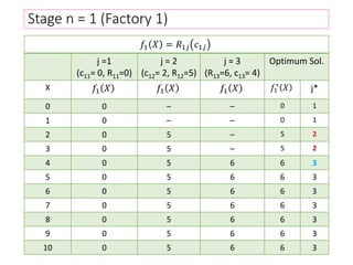
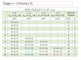
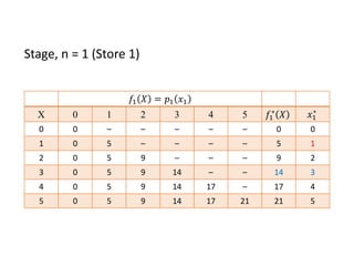
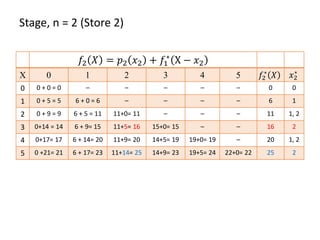
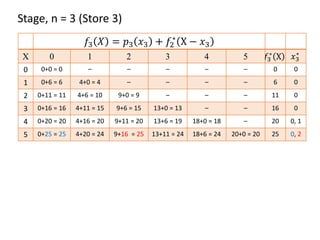
Operations Research
Course Code: IPE 3103
Instructor: Md. Rasel Sarkar
Dept. of IPE, RUET, Rajshahi, Bangladesh
Academic Year: 2020-21
Chapter 10
Dynamic programming
Dynamic Program (DP)
 Dynamic programming is a mathematical technique
dealing with the optimization of multistage decision
process.
 Original decisions problem is divided into small sub-
problem (stages) and stages are optimized rather
than simultaneously.
 In contrast to linear programming, there does not
exist a standard mathematical formulation of “the
dynamic programming problem”.
 Dynamic programming is applicable when the sub-
problems are not independent.
Recursive Nature of Dynamic
Programming
 Computations are then carried out recursively
where the optimum solution of one sub-problem is
used as an input to the next sub-problem.
 The optimum solution for the entire problem is at
hand when the last sub-problem is solved.
 The manner in which the recursive computations
are carried out depends on how the original
problem is decomposed.
Shortest Route Problem
Suppose that we want to select the shortest highway route
between two cities. The network in Figure below provides the
possible routes between the starting city at node 1 and the
destination city at node 7. Where the number on the line
shows distance from one node to another.
First decompose it into stages as delineated by the
vertical dashed lines in Figure. Next, carry out the
computations for each stage separately.
Stage 1
Shortest distance from node 1 to node 2 = 7 miles (from node 1)
Shortest distance from node 1 to node 3 = 8 miles (from node 1)
Shortest distance from node 1 to node 4 = 5 miles (from node 1)
Stage 2 (n=2)
Node 5 can be reached from nodes 2, 3, and 4. Thus –
shortest distance
to node x5
= min
j=2,3,4
{ distance from
node xj to x5
+ shortest distance
to node xj
}
Let,
f*n(xi) be the shortest distance to node xi at stage n
d(xj, xi) as the distance from node xj to node xi.
𝑥𝑗 = all possible routes to node xi.
Now above eqn. can be mathematically expressed as
f*2(x5) = min
j=2,3,4
{d(xj, x5) + (f1(xj)}
Thus,
shortest distance
to node x5
= min
12 + 7 = 19
8 + 8 = 16
7 + 5 = 12
= 12 miles (from node 4)
Node 6 can be reached from nodes 3 and 4. Thus –
shortest distance
to node x6
= min
j=3,4
{ distance from
node xj to x6
+ shortest distance
to node xj
}
= min
9 + 8 = 17
13 + 5 = 18
= 17 miles (from node 3)
Stage 3
The destination node 7 can be reached from either node 5
or 6.
shortest distance
to node x7
= min
j=5,6
distance from
node xj to x7
+ shortest distance
to node xj
= min
9 + 12 = 21
6 + 17 = 23
= 21 miles (from node 5)
Shortest distance from node 1 to node 7 = 21 miles.
Thus, the shortest route is 1 → 4 → 5 → 7.
Recursive equation
The DP recursive equation is defined as –
𝑓0 𝑥1 = 0
𝑓𝑛
∗ 𝑥𝑖 = min 𝑑 𝑥𝑗, 𝑥𝑖 + 𝑓𝑛−1
∗
(𝑥𝑗) , for 𝑛 = 2, 3,…
Principle of optimality
The principle of optimality is the basic principle of
dynamic programming, which was developed by
Richard Bellman that:
“An optimal policy has the property that whatever
the initial conditions and decisions are the remaining
stages constitute an optimal policy regardless of the
policy adopted in all preceding stages”
Capital budgeting problem
Consider the capital budgeting problem where three
existing factories, each being considered for possible
expansion. Factories 1, 2 and 3 have three, four and
two alternative plans for expansion respectively. The
expected additional costs and the corresponding
revenues for jth plan of the nth factory are given by cnj
and Rnj. The objective of the decision problem is to
select a plan j for each factory n which will maximize
the total revenue. The cost of the selected set of
plans should not exceed the total available capital, C.
The data of the problem is tabulated below. All costs
and revenue are scaled by 10-3.
Assume the total capital available is C = 10.
Factory, n n = 1 n = 2 n = 3
Plan, j c1j R1j c2j R2j c3j R3j
1 0 0 0 0 0 0
2 2 5 5 8 1 3
3 4 6 6 9 – –
4 – – 8 12 – –
Recursive equation:
𝑓𝑛
∗ 𝑋 = 𝑚𝑎𝑥
0≤ 𝑐𝑛𝑗≤ 𝑋
{𝑅𝑛𝑗 𝑐𝑛𝑗 + 𝑓𝑛−1
∗
(𝑋 − 𝑐𝑛𝑗)}
Where
X = amounts available for allocation.
𝑓𝑛
∗
𝑋 = the maximum return from allocating X
dollars at nth stage.
𝑐𝑛𝑗 = the decision variable, denote the amount
allocated to jth plan of nth stage.
𝑅𝑛𝑗 𝑐𝑛𝑗 = return from the jth plan on the nth stage.
Stage n = 1 (Factory 1)
𝑓1 𝑋 = 𝑅1𝑗 𝑐1𝑗
j =1
(c11= 0, R11=0)
j = 2
(c12= 2, R12=5)
j = 3
(R13=6, c13= 4)
Optimum Sol.
X 𝑓1 𝑋 𝑓1 𝑋 𝑓1 𝑋 𝑓1
∗
𝑋 j*
0 0 – – 0 1
1 0 – – 0 1
2 0 5 – 5 2
3 0 5 – 5 2
4 0 5 6 6 3
5 0 5 6 6 3
6 0 5 6 6 3
7 0 5 6 6 3
8 0 5 6 6 3
9 0 5 6 6 3
10 0 5 6 6 3
Stage n = 2 (Factory 2)
𝑓2 𝑋 = 𝑅2𝑗 𝑐2𝑗 + 𝑓 ∗1 (𝑋 − 𝑐2𝑗)
j =1
(c21= 0, R21= 0)
j = 2
(c22= 5, R22 = 8)
j = 3
(c23= 6, R23=9)
j = 4
(c24= 8, R23=12)
Optimum
Solution
X 𝑓2 𝑋 𝑓2 𝑋 𝑓2 𝑋 𝑓2 𝑋 𝑓2
∗
𝑋 j*
0 0 + 0 = 0 – – – 0 1
1 0 + 0 = 0 – – – 0 1
2 0 + 5 = 5 – – – 5 1
3 0 + 5 = 5 – – – 5 1
4 0 + 6 = 6 – – – 6 1
5 0 + 6 = 6 8 + 0 = 8 – – 8 2
6 0 + 6 = 6 8 + 0 = 8 9 + 0 = 9 – 9 3
7 0 + 6 = 6 8 + 5 = 13 9 + 0 = 9 – 13 2
8 0 + 6 = 6 8 + 5 = 13 9 + 5 = 14 12 + 0 = 12 14 3
9 0 + 6 = 6 8 + 6 = 14 9 + 5 = 14 12 + 0 = 12 14 2, 3
10 0 + 6 = 6 8 + 6 = 14 9 + 6 = 15 12 + 5 = 17 17 4
Stage n = 3 (Factory 3)
𝑓3 𝑋 = 𝑅3𝑗 𝑐3𝑗 + 𝑓2 (𝑋 − 𝑐3𝑗)*
j =1
(c31 = 0, R31 = 0)
j = 2
(c32= 1, R32 = 3)
Optimum Solution
X 𝑓2 𝑋 𝑓2 𝑋 𝑓3
∗
𝑋 j*
0 0 + 0 = 0 – 0 1
1 0 + 0 = 0 3 + 0 = 3 3 2
2 0 + 5 = 5 3 + 0 = 3 5 1
3 0 + 5 = 5 3 + 5 = 8 8 2
4 0 + 6 = 6 3 + 5 = 8 8 2
5 0 + 8 = 8 3 + 6 = 9 9 2
6 0 + 9 = 9 3 + 8 = 11 11 2
7 0 + 13 = 13 3 + 9 = 12 13 1
8 0 + 14 = 14 3 + 13 = 16 16 2
9 0 + 14 = 14 3 + 14 = 17 17 2
10 0 + 17 = 17 3 + 14 = 17 17 1, 2
Optimal profit = 17
Optimal Policy:
Factory 1 Factory 2 Factory 3
Option 1 2 4 1
Option 2 3 2 2
Option 3 2 3 2
Example
(Liberman)
The owner of a chain of three grocery stores has
purchased five crates of fresh strawberries. The
estimated probability distribution of potential sales
of the strawberries before spoilage differs among the
three stores. Therefore, the owner wants to know
how to allocate five crates to the three stores to
maximize expected profit. For administrative
reasons, the owner does not wish to split crates
between stores. However, he is willing to distribute
no crates to any of his stores.
The following table gives the estimated expected
profit at each store when it is allocated various
numbers of crates:
Use dynamic programming to determine how many
of the five crates should be assigned to each of the
three stores to maximize the total expected profit.
Solution
Let , The decision variables xn (n = 1, 2, 3) are the
number of crates to allocate to stage (store) n.
X = number of crates available for allocation to different
stores.
pn(xn) = be the profit from allocating xn crates to store n.
𝑓𝑛 𝑋 = profit from allocating X crates to store, n
𝑓𝑛
∗
𝑋 = Optimal profit from allocating X crates to store, n
Now get,
𝑓𝑛 𝑋 = 𝑝𝑛 𝑥𝑛 + 𝑓𝑛−1
∗
𝑋 − 𝑥𝑛
Consequently, the recursive relationship is
for n = 1, 2, 3
𝑥𝑛 = 0, 1, 2 … . 𝑋
where 𝑓𝑛
∗ 𝑋 = max 𝑓𝑛
∗ 𝑋 − 𝑥𝑛
𝑓𝑛
∗ 𝑋 = max { 𝑝𝑛 𝑥𝑛 + 𝑓𝑛−1
∗
𝑋 − 𝑥𝑛 }
𝑥𝑛 = 0, 1, 2 … . 𝑋
𝑓1 𝑋 = 𝑝1 𝑥1
X 0 1 2 3 4 5 𝑓1
∗
𝑋 𝑥1
∗
0 0 – – – – – 0 0
1 0 5 – – – – 5 1
2 0 5 9 – – – 9 2
3 0 5 9 14 – – 14 3
4 0 5 9 14 17 – 17 4
5 0 5 9 14 17 21 21 5
Stage, n = 1 (Store 1)
Stage, n = 2 (Store 2)
𝑓2 𝑋 = 𝑝2 𝑥2 + 𝑓1
∗
X − 𝑥2
X 0 1 2 3 4 5 𝑓2
∗
𝑋 𝑥2
∗
0 0 + 0 = 0 – – – – – 0 0
1 0 + 5 = 5 6 + 0 = 6 – – – – 6 1
2 0 + 9 = 9 6 + 5 = 11 11+0= 11 – – – 11 1, 2
3 0+14 = 14 6 + 9= 15 11+5= 16 15+0= 15 – – 16 2
4 0+17= 17 6 + 14= 20 11+9= 20 14+5= 19 19+0= 19 – 20 1, 2
5 0 +21= 21 6 + 17= 23 11+14= 25 14+9= 23 19+5= 24 22+0= 22 25 2
Stage, n = 3 (Store 3)
𝑓3 𝑋 = 𝑝3 𝑥3 + 𝑓2
∗
X − 𝑥3
X 0 1 2 3 4 5 𝑓3
∗
X 𝑥3
∗
0 0+0 = 0 – – – – – 0 0
1 0+6 = 6 4+0 = 4 – – – – 6 0
2 0+11 = 11 4+6 = 10 9+0 = 9 – – – 11 0
3 0+16 = 16 4+11 = 15 9+6 = 15 13+0 = 13 – – 16 0
4 0+20 = 20 4+16 = 20 9+11 = 20 13+6 = 19 18+0 = 18 – 20 0, 1
5 0+25 = 25 4+20 = 24 9+16 = 25 13+11 = 24 18+6 = 24 20+0 = 20 25 0, 2
Optimal Solution
Optimal profit = 25
Optimal Policy:
Store 1 Store 2 Store 3
Option 1 3 2 0
Option 2 1 2 2

Chapter 12 Dynamic programming.pptx

  • 1.
    Operations Research Course Code:IPE 3103 Instructor: Md. Rasel Sarkar Dept. of IPE, RUET, Rajshahi, Bangladesh Academic Year: 2020-21 Chapter 10 Dynamic programming
  • 2.
    Dynamic Program (DP) Dynamic programming is a mathematical technique dealing with the optimization of multistage decision process.  Original decisions problem is divided into small sub- problem (stages) and stages are optimized rather than simultaneously.  In contrast to linear programming, there does not exist a standard mathematical formulation of “the dynamic programming problem”.  Dynamic programming is applicable when the sub- problems are not independent.
  • 3.
    Recursive Nature ofDynamic Programming  Computations are then carried out recursively where the optimum solution of one sub-problem is used as an input to the next sub-problem.  The optimum solution for the entire problem is at hand when the last sub-problem is solved.  The manner in which the recursive computations are carried out depends on how the original problem is decomposed.
  • 4.
    Shortest Route Problem Supposethat we want to select the shortest highway route between two cities. The network in Figure below provides the possible routes between the starting city at node 1 and the destination city at node 7. Where the number on the line shows distance from one node to another.
  • 5.
    First decompose itinto stages as delineated by the vertical dashed lines in Figure. Next, carry out the computations for each stage separately.
  • 6.
    Stage 1 Shortest distancefrom node 1 to node 2 = 7 miles (from node 1) Shortest distance from node 1 to node 3 = 8 miles (from node 1) Shortest distance from node 1 to node 4 = 5 miles (from node 1)
  • 7.
    Stage 2 (n=2) Node5 can be reached from nodes 2, 3, and 4. Thus – shortest distance to node x5 = min j=2,3,4 { distance from node xj to x5 + shortest distance to node xj } Let, f*n(xi) be the shortest distance to node xi at stage n d(xj, xi) as the distance from node xj to node xi. 𝑥𝑗 = all possible routes to node xi. Now above eqn. can be mathematically expressed as f*2(x5) = min j=2,3,4 {d(xj, x5) + (f1(xj)}
  • 8.
    Thus, shortest distance to nodex5 = min 12 + 7 = 19 8 + 8 = 16 7 + 5 = 12 = 12 miles (from node 4) Node 6 can be reached from nodes 3 and 4. Thus – shortest distance to node x6 = min j=3,4 { distance from node xj to x6 + shortest distance to node xj } = min 9 + 8 = 17 13 + 5 = 18 = 17 miles (from node 3)
  • 9.
    Stage 3 The destinationnode 7 can be reached from either node 5 or 6. shortest distance to node x7 = min j=5,6 distance from node xj to x7 + shortest distance to node xj = min 9 + 12 = 21 6 + 17 = 23 = 21 miles (from node 5) Shortest distance from node 1 to node 7 = 21 miles. Thus, the shortest route is 1 → 4 → 5 → 7.
  • 10.
    Recursive equation The DPrecursive equation is defined as – 𝑓0 𝑥1 = 0 𝑓𝑛 ∗ 𝑥𝑖 = min 𝑑 𝑥𝑗, 𝑥𝑖 + 𝑓𝑛−1 ∗ (𝑥𝑗) , for 𝑛 = 2, 3,…
  • 11.
    Principle of optimality Theprinciple of optimality is the basic principle of dynamic programming, which was developed by Richard Bellman that: “An optimal policy has the property that whatever the initial conditions and decisions are the remaining stages constitute an optimal policy regardless of the policy adopted in all preceding stages”
  • 12.
    Capital budgeting problem Considerthe capital budgeting problem where three existing factories, each being considered for possible expansion. Factories 1, 2 and 3 have three, four and two alternative plans for expansion respectively. The expected additional costs and the corresponding revenues for jth plan of the nth factory are given by cnj and Rnj. The objective of the decision problem is to select a plan j for each factory n which will maximize the total revenue. The cost of the selected set of plans should not exceed the total available capital, C.
  • 13.
    The data ofthe problem is tabulated below. All costs and revenue are scaled by 10-3. Assume the total capital available is C = 10. Factory, n n = 1 n = 2 n = 3 Plan, j c1j R1j c2j R2j c3j R3j 1 0 0 0 0 0 0 2 2 5 5 8 1 3 3 4 6 6 9 – – 4 – – 8 12 – –
  • 14.
    Recursive equation: 𝑓𝑛 ∗ 𝑋= 𝑚𝑎𝑥 0≤ 𝑐𝑛𝑗≤ 𝑋 {𝑅𝑛𝑗 𝑐𝑛𝑗 + 𝑓𝑛−1 ∗ (𝑋 − 𝑐𝑛𝑗)} Where X = amounts available for allocation. 𝑓𝑛 ∗ 𝑋 = the maximum return from allocating X dollars at nth stage. 𝑐𝑛𝑗 = the decision variable, denote the amount allocated to jth plan of nth stage. 𝑅𝑛𝑗 𝑐𝑛𝑗 = return from the jth plan on the nth stage.
  • 15.
    Stage n =1 (Factory 1) 𝑓1 𝑋 = 𝑅1𝑗 𝑐1𝑗 j =1 (c11= 0, R11=0) j = 2 (c12= 2, R12=5) j = 3 (R13=6, c13= 4) Optimum Sol. X 𝑓1 𝑋 𝑓1 𝑋 𝑓1 𝑋 𝑓1 ∗ 𝑋 j* 0 0 – – 0 1 1 0 – – 0 1 2 0 5 – 5 2 3 0 5 – 5 2 4 0 5 6 6 3 5 0 5 6 6 3 6 0 5 6 6 3 7 0 5 6 6 3 8 0 5 6 6 3 9 0 5 6 6 3 10 0 5 6 6 3
  • 16.
    Stage n =2 (Factory 2) 𝑓2 𝑋 = 𝑅2𝑗 𝑐2𝑗 + 𝑓 ∗1 (𝑋 − 𝑐2𝑗) j =1 (c21= 0, R21= 0) j = 2 (c22= 5, R22 = 8) j = 3 (c23= 6, R23=9) j = 4 (c24= 8, R23=12) Optimum Solution X 𝑓2 𝑋 𝑓2 𝑋 𝑓2 𝑋 𝑓2 𝑋 𝑓2 ∗ 𝑋 j* 0 0 + 0 = 0 – – – 0 1 1 0 + 0 = 0 – – – 0 1 2 0 + 5 = 5 – – – 5 1 3 0 + 5 = 5 – – – 5 1 4 0 + 6 = 6 – – – 6 1 5 0 + 6 = 6 8 + 0 = 8 – – 8 2 6 0 + 6 = 6 8 + 0 = 8 9 + 0 = 9 – 9 3 7 0 + 6 = 6 8 + 5 = 13 9 + 0 = 9 – 13 2 8 0 + 6 = 6 8 + 5 = 13 9 + 5 = 14 12 + 0 = 12 14 3 9 0 + 6 = 6 8 + 6 = 14 9 + 5 = 14 12 + 0 = 12 14 2, 3 10 0 + 6 = 6 8 + 6 = 14 9 + 6 = 15 12 + 5 = 17 17 4
  • 17.
    Stage n =3 (Factory 3) 𝑓3 𝑋 = 𝑅3𝑗 𝑐3𝑗 + 𝑓2 (𝑋 − 𝑐3𝑗)* j =1 (c31 = 0, R31 = 0) j = 2 (c32= 1, R32 = 3) Optimum Solution X 𝑓2 𝑋 𝑓2 𝑋 𝑓3 ∗ 𝑋 j* 0 0 + 0 = 0 – 0 1 1 0 + 0 = 0 3 + 0 = 3 3 2 2 0 + 5 = 5 3 + 0 = 3 5 1 3 0 + 5 = 5 3 + 5 = 8 8 2 4 0 + 6 = 6 3 + 5 = 8 8 2 5 0 + 8 = 8 3 + 6 = 9 9 2 6 0 + 9 = 9 3 + 8 = 11 11 2 7 0 + 13 = 13 3 + 9 = 12 13 1 8 0 + 14 = 14 3 + 13 = 16 16 2 9 0 + 14 = 14 3 + 14 = 17 17 2 10 0 + 17 = 17 3 + 14 = 17 17 1, 2
  • 18.
    Optimal profit =17 Optimal Policy: Factory 1 Factory 2 Factory 3 Option 1 2 4 1 Option 2 3 2 2 Option 3 2 3 2
  • 19.
    Example (Liberman) The owner ofa chain of three grocery stores has purchased five crates of fresh strawberries. The estimated probability distribution of potential sales of the strawberries before spoilage differs among the three stores. Therefore, the owner wants to know how to allocate five crates to the three stores to maximize expected profit. For administrative reasons, the owner does not wish to split crates between stores. However, he is willing to distribute no crates to any of his stores.
  • 20.
    The following tablegives the estimated expected profit at each store when it is allocated various numbers of crates: Use dynamic programming to determine how many of the five crates should be assigned to each of the three stores to maximize the total expected profit.
  • 21.
    Solution Let , Thedecision variables xn (n = 1, 2, 3) are the number of crates to allocate to stage (store) n. X = number of crates available for allocation to different stores. pn(xn) = be the profit from allocating xn crates to store n. 𝑓𝑛 𝑋 = profit from allocating X crates to store, n 𝑓𝑛 ∗ 𝑋 = Optimal profit from allocating X crates to store, n
  • 22.
    Now get, 𝑓𝑛 𝑋= 𝑝𝑛 𝑥𝑛 + 𝑓𝑛−1 ∗ 𝑋 − 𝑥𝑛 Consequently, the recursive relationship is for n = 1, 2, 3 𝑥𝑛 = 0, 1, 2 … . 𝑋 where 𝑓𝑛 ∗ 𝑋 = max 𝑓𝑛 ∗ 𝑋 − 𝑥𝑛 𝑓𝑛 ∗ 𝑋 = max { 𝑝𝑛 𝑥𝑛 + 𝑓𝑛−1 ∗ 𝑋 − 𝑥𝑛 } 𝑥𝑛 = 0, 1, 2 … . 𝑋
  • 23.
    𝑓1 𝑋 =𝑝1 𝑥1 X 0 1 2 3 4 5 𝑓1 ∗ 𝑋 𝑥1 ∗ 0 0 – – – – – 0 0 1 0 5 – – – – 5 1 2 0 5 9 – – – 9 2 3 0 5 9 14 – – 14 3 4 0 5 9 14 17 – 17 4 5 0 5 9 14 17 21 21 5 Stage, n = 1 (Store 1)
  • 24.
    Stage, n =2 (Store 2) 𝑓2 𝑋 = 𝑝2 𝑥2 + 𝑓1 ∗ X − 𝑥2 X 0 1 2 3 4 5 𝑓2 ∗ 𝑋 𝑥2 ∗ 0 0 + 0 = 0 – – – – – 0 0 1 0 + 5 = 5 6 + 0 = 6 – – – – 6 1 2 0 + 9 = 9 6 + 5 = 11 11+0= 11 – – – 11 1, 2 3 0+14 = 14 6 + 9= 15 11+5= 16 15+0= 15 – – 16 2 4 0+17= 17 6 + 14= 20 11+9= 20 14+5= 19 19+0= 19 – 20 1, 2 5 0 +21= 21 6 + 17= 23 11+14= 25 14+9= 23 19+5= 24 22+0= 22 25 2
  • 25.
    Stage, n =3 (Store 3) 𝑓3 𝑋 = 𝑝3 𝑥3 + 𝑓2 ∗ X − 𝑥3 X 0 1 2 3 4 5 𝑓3 ∗ X 𝑥3 ∗ 0 0+0 = 0 – – – – – 0 0 1 0+6 = 6 4+0 = 4 – – – – 6 0 2 0+11 = 11 4+6 = 10 9+0 = 9 – – – 11 0 3 0+16 = 16 4+11 = 15 9+6 = 15 13+0 = 13 – – 16 0 4 0+20 = 20 4+16 = 20 9+11 = 20 13+6 = 19 18+0 = 18 – 20 0, 1 5 0+25 = 25 4+20 = 24 9+16 = 25 13+11 = 24 18+6 = 24 20+0 = 20 25 0, 2
  • 26.
    Optimal Solution Optimal profit= 25 Optimal Policy: Store 1 Store 2 Store 3 Option 1 3 2 0 Option 2 1 2 2