Download as PDF, PPTX


![خان سنور Algorithm Analysis
Matrix Chain Multiplication
13x15 05x89 89x03 03x34
1 2 3 4
1 0
2 0
3 0
4 0
m[1,1] m[2, 2] m[3, 3] m[4, 4]
m
A CB D](https://image.slidesharecdn.com/dynamicprogramming-190528012358/85/Dynamic-programming-13-320.jpg)
![خان سنور Algorithm Analysis
Matrix Chain Multiplication
1 2 3 4
1 0 5785
2 0 1335
3 0 9078
4 0
m[1, 2] m[2, 3] m[3, 4]
m
m[A, B] m[B, C] m[C, D]
m
A CB D
13x05 05x89 89x03 03x34
13x05 05x89 05x89 89x03 89x03 03x34
13x05x89 05x89x3 89x3x4
5785 1335 9078](https://image.slidesharecdn.com/dynamicprogramming-190528012358/85/Dynamic-programming-14-320.jpg)
![خان سنور Algorithm Analysis
Matrix Chain Multiplication
1 2 3 4
1 0 5785 1530
2 0 1335
3 0 9078
4 0
m[1, 3]
m
A.(B.C) (A.B).C
m
A CB D
13x05 05x89 89x03 03x34
2 Possibilities
13x05 05x89 89x03
1530
m[1, 1] m[2,3] 13 x 5 x 3
Cost A Cost B.C Cost A.B.C = 13x5x3
0 + 1335 + 195
13x05 05x89 89x03
9256
m[1, 2] m[3,3] 13 x 89x 3
5785 + 0 + 3471](https://image.slidesharecdn.com/dynamicprogramming-190528012358/85/Dynamic-programming-15-320.jpg)
![خان سنور Algorithm Analysis
Matrix Chain Multiplication
1 2 3 4
1 0 5785 1530
2 0 1335 1845
3 0 9078
4 0
m[1, 3]
m
B.(C.D) (B.C).D
m
A CB D
13x05 05x89 89x03 03x34
2 Possibilities
05x89 89x03 03x34
24208
m[2, 2] m[3, 4] 05 x 89 x 34
Cost B Cost C.D Cost B.C.D = 05x89x34
0 + 9078 + 15130
05x89 89x03 03x34
1845
m[2, 3] m[4, 4] 5 x 3 x 34
1330 + 0 + 510](https://image.slidesharecdn.com/dynamicprogramming-190528012358/85/Dynamic-programming-16-320.jpg)
![خان سنور Algorithm Analysis
Matrix Chain Multiplication
•m[1, 4]
m[1, 4] = min{m[1,1] + m[2,4], 13 x 5 x 34,
m[1, 2] + m[3, 4] + 13 x 89 x 34,
m[1, 3] + m[4, 4] + 13 x 3 x 34 }](https://image.slidesharecdn.com/dynamicprogramming-190528012358/85/Dynamic-programming-17-320.jpg)
![خان سنور Algorithm Analysis
Matrix Chain Multiplication
•m[1, 4]
m[1, 4] = min{A. (B. C. D), (A.B).(C.D),(A.B.C).D}](https://image.slidesharecdn.com/dynamicprogramming-190528012358/85/Dynamic-programming-18-320.jpg)
![خان سنور Algorithm Analysis
Matrix Chain Multiplication
•m[1, 4]
m[1, 4] = min{0 + 1845 + 2210,
5789 + 78 + 39338,
1530 + 0 + 1326}](https://image.slidesharecdn.com/dynamicprogramming-190528012358/85/Dynamic-programming-19-320.jpg)
![خان سنور Algorithm Analysis
Matrix Chain Multiplication
•m[1, 4]
m[1, 4] = min{4055, 54201, 2856}
WHAT IS MIN? 2856
1 2 3 4
1 0 5785 1530 2856
2 0 1335 1845
3 0 9078
4 0
mm](https://image.slidesharecdn.com/dynamicprogramming-190528012358/85/Dynamic-programming-20-320.jpg)
![خان سنور Algorithm Analysis
Formula
•m[i, j] = min{m(I, k) + m(k+1, j) + di-1xdkxdj}](https://image.slidesharecdn.com/dynamicprogramming-190528012358/85/Dynamic-programming-21-320.jpg)

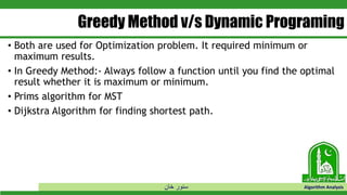
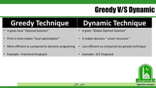
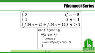
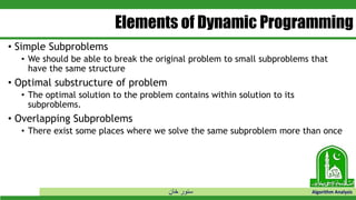
This document discusses greedy algorithms and dynamic programming. It explains that greedy algorithms find local optimal solutions at each step, while dynamic programming finds global optimal solutions by considering all possibilities. The document also provides examples of problems solved using each approach, such as Prim's algorithm and Dijkstra's algorithm for greedy, and knapsack problems for dynamic programming. It then discusses the matrix chain multiplication problem in detail to illustrate how a dynamic programming solution works by breaking the problem into overlapping subproblems.