Design and Analysis Algorithms.pdf

DESIGN AND ANALYSIS OF ALGORITHMS Page 1
DIGITAL NOTES
ON
DESIGN AND ANALYSIS OF ALGORITHMS
B.TECH II YEAR - II SEM
(2017-18)
DEPARTMENT OF INFORMATION TECHNOLO
MALLA REDDY COLLEGE OF ENGINEERING & TECHNOLOGY
(Autonomous Institution – UGC, Govt. of India)
(Affiliated to JNTUH, Hyderabad, Approved by AICTE - Accredited by NBA & NAAC – ‘A’ Grade - ISO 9001:2015 Certified)
Maisammaguda, Dhulapally (Post Via. Hakimpet), Secunderabad – 500100, Telangana State, INDIA.

DEPARTMENT OF INFORMATION TECHNOLOGY
SYLLABUS
MALLA REDDY COLLEGE OF ENGINEERING AND
TECHNOLOGY
II Year B.Tech IT – II Sem L T /P/D C
4 - / - / - 3
(R15A0508)DESIGN AND ANALYSIS OF ALGORITHMS
Objectives:
 To analyze performance of algorithms.
 To choose the appropriate data structure and algorithm design method for a specified
application.
 To understand how the choice of data structures and algorithm design methods
impacts the performance of programs.
 To solve problems using algorithm design methods such as the greedy method, divide
and conquer, dynamic programming, backtracking and branch and bound.
 Prerequisites (Subjects) Data structures, Mathematical foundations of computer
science.
UNIT I:
Introduction: Algorithm, Psuedo code for expressing algorithms, Performance Analysis-
Space complexity, Time complexity, Asymptotic Notation- Big oh notation, Omega notation,
Theta notation and Little oh notation, Probabilistic analysis, Amortized analysis.
Divide and conquer: General method, applications-Binary search, Quick sort, Merge sort,
Strassen’s matrix multiplication.
UNIT II:
Searching and Traversal Techniques: Efficient non - recursive binary tree traversal
algorithm, Disjoint set operations, union and find algorithms, Spanning trees, Graph
traversals - Breadth first search and Depth first search, AND / OR graphs, game trees,
Connected Components, Bi - connected components. Disjoint Sets- disjoint set operations,
union and find algorithms, spanning trees, connected components and biconnected
components.
UNIT III:
Greedy method: General method, applications - Job sequencing with deadlines, 0/1
knapsack problem, Minimum cost spanning trees, Single source shortest path problem.
Dynamic Programming: General method, applications-Matrix chain multiplication, Optimal
binary search trees, 0/1 knapsack problem, All pairs shortest path problem, Travelling sales
person problem, Reliability design.

UNIT IV:
Backtracking: General method, applications-n-queen problem, sum of subsets problem,
graph coloring, Hamiltonian cycles.
Branch and Bound: General method, applications - Travelling sales person problem,0/1
knapsack problem- LC Branch and Bound solution, FIFO Branch and Bound solution.
UNIT V:
NP-Hard and NP-Complete problems: Basic concepts, non deterministic algorithms, NP -
Hard and NPComplete classes, Cook’s theorem.
TEXT BOOKS:
1. Fundamentals of Computer Algorithms, Ellis Horowitz,Satraj Sahni
and Rajasekharam,Galgotia publications pvt. Ltd.
2. Foundations of Algorithm, 4th edition, R. Neapolitan and K. Naimipour, Jones and
Bartlett Learning.
3. Design and Analysis of Algorithms, P. H. Dave, H. B. Dave, Pearson Education,
2008.
REFERENCES:
1. Computer Algorithms, Introduction to Design and Analysis, 3rd Edition, Sara Baase,
Allen, Van, Gelder, Pearson Education.
2. Algorithm Design: Foundations, Analysis and Internet examples, M. T. Goodrich and
R. Tomassia, John Wiley and sons.
3. Fundamentals of Sequential and Parallel Algorithm, K. A. Berman and J. L. Paul,
Cengage Learning.
4. Introducation to the Design and Analysis of Algorithms, A. Levitin, Pearson
Education.
5. Introducation to Algorithms, 3rd Edition, T. H. Cormen, C. E. Leiserson, R. L. Rivest,
and C. Stein, PHI Pvt. Ltd.
6. Design and Analysis of algorithm, Aho, Ullman and Hopcroft, Pearson Education,
2004.
Outcomes:
 Be able to analyze algorithms and improve the efficiency of algorithms.
 Apply different designing methods for development of algorithms to realistic
problems, such as divide and conquer, greedy and etc. Ability to understand and
estimate the performance of algorithm.

INDEX
S. No
Unit
Topic Page no
1 I Introduction to Algorithms 5
2 I Divide and Conquer 24
3 II Searching and Traversal Techniques 42
4 III Greedy Method 54
5 III Dynamic Programming 67
6 IV Back Tracking 102
7 IV Branch and Bound 114
8 V NP-Hard and NP-Complete Problems 133
9

UNIT I:
Introduction: Algorithm, Psuedo code for expressing algorithms, Performance Analysis-
Space complexity, Time complexity, Asymptotic Notation- Big oh notation, Omega notation,
Theta notation and Little oh notation, Probabilistic analysis, Amortized analysis.
Divide and conquer: General method, applications-Binary search, Quick sort, Merge sort,
Strassen’s matrix multiplication.
INTRODUCTION TO ALGORITHM
History of Algorithm
• The word algorithm comes from the name of a Persian author, Abu Ja’far Mohammed ibn
Musa al Khowarizmi (c. 825 A.D.), who wrote a textbook on mathematics.
• He is credited with providing the step-by-step rules for adding, subtracting, multiplying,
and dividing ordinary decimal numbers.
• When written in Latin, the name became Algorismus, from which algorithm is but a small
step
• This word has taken on a special signiﬁcance in computer science, where “algorithm” has
come to refer to a method that can be used by a computer for the solution of a problem
• Between 400 and 300 B.C., the great Greek mathematician Euclid invented an algorithm
• Finding the greatest common divisor (gcd) of two positive integers.
• The gcd of X and Y is the largest integer that exactly divides both X and Y .
• Eg.,the gcd of 80 and 32 is 16.
• The Euclidian algorithm, as it is called, is considered to be the first non-trivial algorithm
ever devised.
What is an Algorithm?
Algorithm is a set of steps to complete a task.
For example,
Task: to make a cup of tea.
Algorithm:
· add water and milk to the kettle,
· boil it, add tea leaves,
· Add sugar, and then serve it in cup.
‘’a set of steps to accomplish or complete a task that is described precisely enough that
a computer can run it’’.
Described precisely: very difficult for a machine to know how much water, milk to be
added etc. in the above tea making algorithm.

These algorithms run on computers or computational devices..For example, GPS in our
smartphones, Google hangouts.
GPS uses shortest path algorithm.. Online shopping uses cryptography which uses RSA
algorithm.
• Algorithm Definition1:
• An algorithm is a finite set of instructions that, if followed, accomplishes a particular task.
In addition, all algorithms must satisfy the following criteria:
• Input. Zero or more quantities are externally supplied.
• Output. At least one quantity is produced.
• Definiteness. Each instruction is clear and unambiguous.
• Finiteness. The algorithm terminates after a finite number of steps.
• Effectiveness. Every instruction must be very basic enough and must be
feasible.
• Algorithm Definition2:
• An algorithm is a sequence of unambiguous instructions for solving a problem, i.e., for
obtaining a required output for any legitimate input in a finite amount of time.
• Algorithms that are definite and effective are also called computational procedures.
• A program is the expression of an algorithm in a programming language
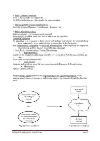
• Algorithms for Problem Solving
The main steps for Problem Solving are:
1. Problem definition
2. Algorithm design / Algorithm specification
3. Algorithm analysis
4. Implementation
5. Testing
6. [Maintenance]

• Step1. Problem Definition
What is the task to be accomplished?
Ex: Calculate the average of the grades for a given student
• Step2.Algorithm Design / Specifications:
Describe: in natural language / pseudo-code / diagrams / etc
• Step3. Algorithm analysis
Space complexity - How much space is required
Time complexity - How much time does it take to run the algorithm
Computer Algorithm
An algorithm is a procedure (a finite set of well-defined instructions) for accomplishing
some tasks which, given an initial state terminate in a defined end-state
The computational complexity and efficient implementation of the algorithm are important
in computing, and this depends on suitable data structures.
• Steps 4,5,6: Implementation, Testing, Maintainance
• Implementation:
Decide on the programming language to use C, C++, Lisp, Java, Perl, Prolog, assembly, etc.
, etc.
Write clean, well documented code
• Test, test, test
Integrate feedback from users, fix bugs, ensure compatibility across different versions
• Maintenance.
Release Updates,fix bugs
Keeping illegal inputs separate is the responsibility of the algorithmic problem, while
treating special classes of unusual or undesirable inputs is the responsibility of the algorithm
itself.

• 4 Distinct areas of study of algorithms:
• How to devise algorithms.  Techniques – Divide & Conquer, Branch and Bound ,
Dynamic Programming
• How to validate algorithms.
• Check for Algorithm that it computes the correct answer for all possible legal inputs. 
algorithm validation.  First Phase
• Second phase  Algorithm to Program  Program Proving or Program Verification
Solution be stated in two forms:
• First Form: Program which is annotated by a set of assertions about the input and output
variables of the program predicate calculus
• Second form: is called a specification
• 4 Distinct areas of study of algorithms (..Contd)
• How to analyze algorithms.
• Analysis of Algorithms or performance analysis refer to the task of determining how
much computing time & storage an algorithm requires
• How to test a program  2 phases 
• Debugging - Debugging is the process of executing programs on sample data sets to
determine whether faulty results occur and, if so, to correct them.
• Proﬁling or performance measurement is the process of executing a correct program on
data sets and measuring the time and space it takes to compute the results
PSEUDOCODE:
• Algorithm can be represented in Text mode and Graphic mode
• Graphical representation is called Flowchart
• Text mode most often represented in close to any High level language such as C,
PascalPseudocode
• Pseudocode: High-level description of an algorithm.
• More structured than plain English.
• Less detailed than a program.
• Preferred notation for describing algorithms.
• Hides program design issues.
• Example of Pseudocode:
• To find the max element of an array
Algorithm arrayMax(A, n)
Input array A of n integers
Output maximum element of A
currentMax  A[0]
for i  1 to n  1 do
if A[i]  currentMax then
currentMax  A[i]

return currentMax
• Control flow
• if … then … [else …]
• while … do …
• repeat … until …
• for … do …
• Indentation replaces braces
• Method declaration
• Algorithm method (arg [, arg…])
• Input …
• Output …
• Method call
• var.method (arg [, arg…])
• Return value
• return expression
• Expressions
• Assignment (equivalent to )
• Equality testing (equivalent to )
• n2
Superscripts and other mathematical formatting allowed
PERFORMANCE ANALYSIS:
• What are the Criteria for judging algorithms that have a more direct relationship to
performance?
• computing time and storage requirements.
• Performance evaluation can be loosely divided into two major phases:
• a priori estimates and
• a posteriori testing.
• refer as performance analysis and performance measurement respectively
• The space complexity of an algorithm is the amount of memory it needs to run to
completion.
• The time complexity of an algorithm is the amount of computer time it needs to run to
completion.
Space Complexity:
• Space Complexity Example:
• Algorithm abc(a,b,c)
{
return a+b++*c+(a+b-c)/(a+b) +4.0;
}

The Space needed by each of these algorithms is seen to be the sum of the following
component.

1.A fixed part that is independent of the characteristics (eg:number,size)of the inputs and
outputs.
The part typically includes the instruction space (ie. Space for the code), space for simple
variable and fixed-size component variables (also called aggregate) space for constants, and
so on.
2. A variable part that consists of the space needed by component variables whose size is
dependent on the particular problem instance being solved, the space needed by referenced
variables (to the extent that is depends on instance characteristics), and the recursion stack
space.

The space requirement s(p) of any algorithm p may therefore be written as,
S(P) = c+ Sp(Instance characteristics)
Where ‘c’ is a constant.
Example 2:
Algorithm sum(a,n)
{
s=0.0;
for I=1 to n do
s= s+a[I];
return s;
}
The problem instances for this algorithm are characterized by n,the number of
elements to be summed. The space needed d by ‘n’ is one word, since it is of
type integer.
The space needed by ‘a’a is the space needed by variables of tyepe array of
floating point numbers.
This is atleast ‘n’ words, since ‘a’ must be large enough to hold the ‘n’
elements to be summed.
So,we obtain Ssum(n)>=(n+s)
• [ n for a[],one each for n,I a& s]
Time Complexity:
• The time T(p) taken by a program P is the sum of the compile time and the
run time(execution time)
• The compile time does not depend on the instance characteristics. Also we may
assume that a compiled program will be run several times without recompilation .This
rum time is denoted by tp(instance characteristics).
• The number of steps any problem statement is assigned depends on the kind of
statement.
• For example, comments à 0 steps.
Assignment statements is 1 steps.

[Which does not involve any calls to other algorithms]
Interactive statement such as for, while & repeat-untilà Control part of the statement.
We introduce a variable, count into the program statement to increment count with
initial value 0.Statement to increment count by the appropriate amount are introduced
into the program.
This is done so that each time a statement in the original program is executes
count is incremented by the step count of that statement.
Algorithm:
Algorithm sum(a,n)
{
s= 0.0;
count = count+1;
for I=1 to n do
{
count =count+1;
s=s+a[I];
count=count+1;
}
count=count+1;
count=count+1;
return s;
}

If the count is zero to start with, then it will be 2n+3 on termination. So each
invocation of sum execute a total of 2n+3 steps.
2. The second method to determine the step count of an algorithm is to build a
table in which we list the total number of steps contributes by each statement.

First determine the number of steps per execution (s/e) of the statement and the
total number of times (ie., frequency) each statement is executed.

By combining these two quantities, the total contribution of all statements, the
step count for the entire algorithm is obtained.
Statement Steps per
execution
Frequency Total
1. Algorithm Sum(a,n)
2.{
3. S=0.0;
4. for I=1 to n do
5. s=s+a[I];
6. return s;
7. }
0
0
1
1
1
1
0
-
-
1
n+1
n
1
-
0
0
1
n+1
n
1
0
Total 2n+3

How to analyse an Algorithm?
Let us form an algorithm for Insertion sort (which sort a sequence of numbers).The pseudo
code for the algorithm is give below.
Pseudo code for insertion Algorithm:
Identify each line of the pseudo code with symbols such as C1, C2 ..
PSeudocode for Insertion Algorithm Line Identification
for j=2 to A length C1
key=A[j] C2
//Insert A[j] into sorted Array A[1.....j-1] C3
i=j-1 C4
while i>0 & A[j]>key C5
A[i+1]=A[i] C6
i=i-1 C7
A[i+1]=key C8
Let Ci be the cost of ith line. Since comment lines will not incur any cost C3=0.
Cost No. Of times
Executed
C1 N
C2 n-1
C3=0 n-1
C4 n-1
C5
C6
C7
C8 n-1
Running time of the algorithm is:
T(n)=C1n+C2(n-1)+0(n-1)+C4(n-1)+C5( )+C6( )+C7( )+
C8(n-1)
Best case:
It occurs when Array is sorted.
All tj values are 1.

T(n)=C1n+C2(n-1)+0 (n-1)+C4(n-1)+C5( ) +C6( )+C7( )+
C8(n-1)
=C1n+C2 (n-1) +0 (n-1) +C4 (n-1) +C5 + C8 (n-1)
= (C1+C2+C4+C5+ C8) n-(C2+C4+C5+ C8)
· Which is of the form an+b.
· Linear function of n.
So, linear growth.
Worst case:
It occurs when Array is reverse sorted, and tj =j
T(n)=C1n + C2(n-1)+0 (n-1)+C4(n-1)+C5( ) +C6( )+C7( ) +
C8(n-1)
=C1n+C2(n-1)+C4(n-1)+C5( ) +C6( )+C7( )+ C8(n-1)
which is of the form an2
+bn+c
Quadratic function. So in worst case insertion set grows in n2.
Why we concentrate on worst-case running time?
· The worst-case running time gives a guaranteed upper bound on the running time for
any input.
· For some algorithms, the worst case occurs often. For example, when searching, the
worst case often occurs when the item being searched for is not present, and searches
for absent items may be frequent.
· Why not analyze the average case? Because it’s often about as bad as the worst case.
Order of growth:
It is described by the highest degree term of the formula for running time. (Drop lower-order
terms. Ignore the constant coefficient in the leading term.)
Example: We found out that for insertion sort the worst-case running time is of the form
an2
+ bn + c.
Drop lower-order terms. What remains is an2.Ignore constant coefficient. It results in n2
.But
we cannot say that the worst-case running time T(n) equals n2
.Rather It grows like n2
. But it
doesn’t equal n2
.We say that the running time is Θ (n2
) to capture the notion that the order of
growth is n2
.

We usually consider one algorithm to be more efficient than another if its worst-case
running time has a smaller order of growth.
Complexity of Algorithms
The complexity of an algorithm M is the function f(n) which gives the running time and/or
storage space requirement of the algorithm in terms of the size ‘n’ of the input data. Mostly,
the storage space required by an algorithm is simply a multiple of the data size ‘n’.
Complexity shall refer to the running time of the algorithm.
The function f(n), gives the running time of an algorithm, depends not only on the size ‘n’ of
the input data but also on the particular data. The complexity function f(n) for certain cases
are:
1. Best Case : The minimum possible value of f(n) is called the best case.
2. Average Case : The expected value of f(n).
3. Worst Case : The maximum value of f(n) for any key possible input.
ASYMPTOTIC NOTATION
 Formal way notation to speak about functions and classify them
The following notations are commonly use notations in performance analysis and used to
characterize the complexity of an algorithm:
1. Big–OH (O) ,
2. Big–OMEGA (Ω),
3. Big–THETA (Θ) and
4. Little–OH (o)
Asymptotic Analysis of Algorithms:
Our approach is based on the asymptotic complexity measure. This means that we don’t try to
count the exact number of steps of a program, but how that number grows with the size of the
input to the program. That gives us a measure that will work for different operating systems,
compilers and CPUs. The asymptotic complexity is written using big-O notation.
· It is a way to describe the characteristics of a function in the limit.
· It describes the rate of growth of functions.
· Focus on what’s important by abstracting away low-order terms and constant factors.
· It is a way to compare “sizes” of functions:
O≈ ≤

Ω≈ ≥
Θ ≈ =
o ≈ <
ω ≈ >
Time complexity Name Example
O(1) Constant Adding an element to the
front of a linked list
O(logn) Logarithmic Finding an element in a
sorted array
O (n) Linear Finding an element in an
unsorted array
O(nlog n) Linear Logarithmic Sorting n items
by ‘divide-and-conquer’-
Mergesort
O(n2
) Quadratic Shortest path between two
nodes in a graph
O(n3
) Cubic Matrix Multiplication
O(2n
) Exponential The Towers of Hanoi
problem
Big ‘oh’: the function f(n)=O(g(n)) iff there exist positive constants c and no such that
f(n)<=c*g(n) for all n, n>= no.
Omega: the function f(n)=(g(n)) iff there exist positive constants c and no such that
f(n) >= c*g(n) for all n, n >= no.
Theta: the function f(n)=(g(n)) iff there exist positive constants c1,c2 and no such that c1
g(n) <= f(n) <= c2 g(n) for all n, n >= no
Big-O Notation
This notation gives the tight upper bound of the given function. Generally we represent it as
f(n) = O(g (11)). That means, at larger values of n, the upper bound off(n) is g(n). For
example, if f(n) = n4
+ 100n2
+ 10n + 50 is the given algorithm, then n4
is g(n). That means
g(n) gives the maximum rate of growth for f(n) at larger values of n.
O —notation deﬁned as O(g(n)) = {f(n): there exist positive constants c and no such that
0 <= f(n) <= cg(n) for all n >= no}. g(n) is an asymptotic tight upper bound for f(n). Our
objective is to give some rate of growth g(n) which is greater than given algorithms rate of
growth f(n).
In general, we do not consider lower values of n. That means the rate of growth at lower
values of n is not important. In the below ﬁgure, no is the point from which we consider the
rate of growths for a given algorithm. Below no the rate of growths may be different.

Note Analyze the algorithms at larger values of n only What this means is, below no we do
not care for rates of growth.
Omega— Ω notation
Similar to above discussion, this notation gives the tighter lower bound of the given
algorithm and we represent it as f(n) = Ω (g(n)). That means, at larger values of n, the
tighter lower bound of f(n) is g
For example, if f(n) = 100n2
+ 10n + 50, g(n) is Ω (n2
).
The . Ω. notation as be defined as Ω (g (n)) = {f(n): there exist positive constants c and
no such that 0 <= cg (n) <= f(n) for all n >= no}. g(n) is an asymptotic lower bound for
f(n). Ω (g (n)) is the set of functions with smaller or same order of growth as f(n).
Theta- Θ notation
This notation decides whether the upper and lower bounds of a given function are same or
not. The average running time of algorithm is always between lower bound and upper bound.

If the upper bound (O) and lower bound (Ω) gives the same result then Θ notation will also
have the same rate of growth. As an example, let us assume that f(n) = 10n + n is the
expression. Then, its tight upper bound g(n) is O(n). The rate of growth in best case is g (n) =
0(n). In this case, rate of growths in best case and worst are same. As a result, the average
case will also be same.
None: For a given function (algorithm), if the rate of growths (bounds) for O and Ω are not
same then the rate of growth Θ case may not be same.
Now consider the deﬁnition of Θ notation It is deﬁned as Θ (g(n)) = {f(71): there exist
positive constants C1, C2 and no such that O<=5 c1g(n) <= f(n) <= c2g(n) for all n >= no}.
g(n) is an asymptotic tight bound for f(n). Θ (g(n)) is the set of functions with the same
order of growth as g(n).
Important Notes
For analysis (best case, worst case and average) we try to give upper bound (O) and lower
bound (Ω) and average running time (Θ). From the above examples, it should also be clear
that, for a given function (algorithm) getting upper bound (O) and lower bound (Ω) and
average running time (Θ) may not be possible always.
For example, if we are discussing the best case of an algorithm, then we try to give upper
bound (O) and lower bound (Ω) and average running time (Θ).
In the remaining chapters we generally concentrate on upper bound (O) because knowing
lower bound (Ω) of an algorithm is of no practical importance and we use 9 notation if upper
bound (O) and lower bound (Ω) are same.
Little Oh Notation
The little Oh is denoted as o. It is defined as : Let, f(n} and g(n} be the non negative
functions then

such that f(n}= o(g{n)} i.e f of n is little Oh of g of n.
f(n) = o(g(n)) if and only if f'(n) = o(g(n)) and f(n) != Θ {g(n))
PROBABILISTIC ANALYSIS
Probabilistic analysis is the use of probability in the analysis of problems.
In order to perform a probabilistic analysis, we must use knowledge of, or make assumptions
about, the distribution of the inputs. Then we analyze our algorithm, computing an average-
case running time, where we take the average over the distribution of the possible inputs.
Basics of Probability Theory
Probability theory has the goal of characterizing the outcomes of natural or conceptual
“experiments.” Examples of such experiments include tossing a coin ten times, rolling a die
three times, playing a lottery, gambling, picking a ball from an urn containing white and red
balls, and so on
Each possible outcome of an experiment is called a sample point and the set of all possible
outcomes is known as the sample space S. In this text we assume that S is finite (such a
sample space is called a discrete sample space). An event E is a subset of the sample space S.
If the sample space consists of n sample points, then there are 2n
possible events.
Definition- Probability: The probability of an event E is defined to be where S is the
sample space.
Then the indicator random variable I {A} associated with event A is defined as
I {A} = 1 if A occurs ;
0 if A does not occur
The probability of event E is denoted as Prob. [E] The complement of E, denoted E, is
defined to be S - E. If E1 and E2 are two events, the probability of E1 or E2 or both
happening is denoted as Prob.[E1 U E2]. The probability of both E1 and E2 occurring at the
same time is denoted as Prob.[E1 0 E2]. The corresponding event is E1 0 E2.
Theorem 1.5
1. Prob.[E] = 1 - Prob.[E].
2. Prob.[E1 U E2] = Prob.[E1] + Prob.[E2] - Prob.[E1 ∩ E2]
<= Prob.[E1] + Prob.[E2]
Expected value of a random variable

The simplest and most useful summary of the distribution of a random variable is the
average” of the values it takes on. The expected value (or, synonymously, expectation or
mean) of a discrete random variable X is
E[X] =
which is well defined if the sum is finite or converges absolutely.
Consider a game in which you flip two fair coins. You earn $3 for each head but lose $2 for
each tail. The expected value of the random variable X representing
your earnings is
E[X] = 6.Pr{2H’s} + 1.Pr{1H,1T} – 4 Pr{2T’s}
= 6(1/4)+1(1/2)-4(1/4)
=1
Any one of these first i candidates is equally likely to be the best-qualified so far. Candidate i
has a probability of 1/i of being better qualified than candidates 1 through i -1 and thus a
probability of 1/i of being hired.
E[Xi]= 1/i
So,
E[X] = E[ ]
=
=
AMORTIZED ANALYSIS
In an amortized analysis, we average the time required to perform a sequence of datastructure
operations over all the operations performed. With amortized analysis, we can show that the
average cost of an operation is small, if we average over a sequence of operations, even
though a single operation within the sequence might be expensive. Amortized analysis differs
from average-case analysis in that probability is not involved; an amortized analysis
guarantees the average performance of each operation in the worst case.
Three most common techniques used in amortized analysis:
1. Aggregate Analysis - in which we determine an upper bound T(n) on the total cost
of a sequence of n operations. The average cost per operation is then T(n)/n. We take
the average cost as the amortized cost of each operation
2. Accounting method – When there is more than one type of operation, each type of
operation may have a different amortized cost. The accounting method overcharges
some operations early in the sequence, storing the overcharge as “prepaid credit” on
specific objects in the data structure. Later in the sequence, the credit pays for
operations that are charged less than they actually cost.

3. Potential method - The potential method maintains the credit as the “potential
energy” of the data structure as a whole instead of associating the credit with
individual objects within the data structure. The potential method, which is like the
accounting method in that we determine the amortized cost of each operation and
may overcharge operations early on to compensate for undercharges later
DIVIDE AND CONQUER
General Method
In divide and conquer method, a given problem is,
i) Divided into smaller subproblems.
ii) These subproblems are solved independently.
iii) Combining all the solutions of subproblems into a solution of the whole.
If the subproblems are large enough then divide and conquer is reapplied.
The generated subproblems are usually of some type as the original problem.
Hence recurssive algorithms are used in divide and conquer strategy.
Pseudo code Representation of Divide and conquer rule for problem “P”
Problem of size N
Subprogram of size
N/2
Subprogram of size
N/2
Solution to
subprogram 1
Solution to
subprogram 2
Solution to the original problem of
size n

Algorithm DAndC(P)
{
if small(P) then return S(P)
else{
divide P into smaller instances P1,P2,P3…Pk;
apply DAndC to each of these subprograms; // means DAndC(P1), DAndC(P2)…..
DAndC(Pk)
return combine(DAndC(P1), DAndC(P2)….. DAndC(Pk));
}
}
//PProblem
//Here small(P) Boolean value function. If it is true, then the function S is
//invoked
Time Complexity of DAndC algorithm:
a,b contants.
This is called the general divide and-conquer recurrence.
Example for GENERAL METHOD:
As an example, let us consider the problem of computing the sum of n numbers a0, ... an-1.
If n > 1, we can divide the problem into two instances of the same problem. They are sum of
the first | n/2|numbers
Compute the sum of the 1st
[n/2] numbers, and then compute the sum of another n/2 numbers.
Combine the answers of two n/2 numbers sum.
i.e.,
a0 + . . . + an-1 =( a0 + ....+ an/2) + (a n/2 + . . . . + an-1)
Assuming that size n is a power of b, to simplify our analysis, we get the following
recurrence for the running time T(n).
T(n)=aT(n/b)+f(n)
This is called the general divide and-conquer recurrence.
f(n) is a function that accounts for the time spent on dividing the problem into smaller ones
and on combining their solutions. (For the summation example, a = b = 2 and f (n) = 1.
Advantages of DAndC:
The time spent on executing the problem using DAndC is smaller than other method.
This technique is ideally suited for parallel computation.
This approach provides an efficient algorithm in computer science.
Master Theorem for Divide and Conquer
In all efficient divide and conquer algorithms we will divide the problem into subproblems,
each of which is some part of the original problem, and then perform some additional work to
compute the ﬁnal answer. As an example, if we consider merge sort [for details, refer Sorting
chapter], it operates on two problems, each of which is half the size of the original, and then
uses O(n) additional work for merging. This gives the running time equation:
T(n) = T(1) if n=1
aT(n/b)+f(n) if n>1

T(n) = 2T( )+ O(n)
The following theorem can be used to determine the running time of divide and conquer
algorithms. For a given program or algorithm, ﬁrst we try to ﬁnd the recurrence relation for
the problem. If the recurrence is of below form then we directly give the answer without
fully solving it.
If the reccurrence is of the form T(n) = aT( ) + Θ (nklogp
n), where a >= 1, b > 1, k >= O
and p is a real number, then we can directly give the answer as:
1) If a > bk
, then T(n) = Θ ( )
2) If a = bk
a. If p > -1, then T(n) = Θ ( )
b. If p = -1, then T(n) = Θ ( )
c. If p < -1, then T(n) = Θ ( s)
3) If a < bk
a. If p >= 0, then T(n) = Θ (nk
logpn
)
b. If p < 0, then T(n) = 0(nk
)
Applications of Divide and conquer rule or algorithm:
 Binary search,
 Quick sort,
 Merge sort,
 Strassen’s matrix multiplication.
Binary search or Half-interval search algorithm:
1. This algorithm finds the position of a specified input value (the search "key") within
an array sorted by key value.
2. In each step, the algorithm compares the search key value with the key value of the
middle element of the array.
3. If the keys match, then a matching element has been found and its index, or position,
is returned.
4. Otherwise, if the search key is less than the middle element's key, then the algorithm
repeats its action on the sub-array to the left of the middle element or, if the search
key is greater, then the algorithm repeats on sub array to the right of the middle
element.
5. If the search element is less than the minimum position element or greater than the
maximum position element then this algorithm returns not found.
Binary search algorithm by using recursive methodology:
Program for binary search (recursive) Algorithm for binary search (recursive)
int binary_search(int A[], int key, int imin, int imax) Algorithm binary_search(A, key, imin, imax)

{
if (imax < imin)
return array is empty;
if(key<imin || K>imax)
return element not in array list
else
{
int imid = (imin +imax)/2;
if (A[imid] > key)
return binary_search(A, key, imin, imid-1);
else if (A[imid] < key)
return binary_search(A, key, imid+1, imax);
else
return imid;
}
}
{
if (imax < imin) then
return “array is empty”;
if(key<imin || K>imax) then
return “element not in array list”
else
{
imid = (imin +imax)/2;
if (A[imid] > key) then
return binary_search(A, key, imin, imid-1);
else if (A[imid] < key) then
return binary_search(A, key, imid+1, imax);
else
return imid;
}
}
Time Complexity:
Data structure:- Array
For successful search Unsuccessful search
Worst case O(log n) or θ(log n)
Average case O(log n) or θ(log n)
Best case O(1) or θ(1)
θ(log n):- for all cases.
Binary search algorithm by using iterative methodology:
Binary search program by using iterative
methodology:
Binary search algorithm by using iterative
methodology:
int binary_search(int A[], int key, int imin, int
imax)
{
while (imax >= imin)
{
int imid = midpoint(imin, imax);
if(A[imid] == key)
return imid;
imin = imid + 1;
else
imax = imid - 1;
}
}
Algorithm binary_search(A, key, imin, imax)
{
While < (imax >= imin)> do
{
int imid = midpoint(imin, imax);
if(A[imid] == key)
return imid;
imin = imid + 1;
else
imax = imid - 1;
}
}
Merge Sort:
The merge sort splits the list to be sorted into two equal halves, and places them in separate
arrays. This sorting method is an example of the DIVIDE-AND-CONQUER paradigm i.e. it
breaks the data into two halves and then sorts the two half data sets recursively, and finally
merges them to obtain the complete sorted list. The merge sort is a comparison sort and has an
algorithmic complexity of O (n log n). Elementary implementations of the merge sort make use of
two arrays - one for each half of the data set. The following image depicts the complete procedure
of merge sort.

Advantages of Merge Sort:
1. Marginally faster than the heap sort for larger sets
2. Merge Sort always does lesser number of comparisons than Quick Sort. Worst case for
merge sort does about 39% less comparisons against quick sort’s average case.
3. Merge sort is often the best choice for sorting a linked list because the slow random-
access performance of a linked list makes some other algorithms (such as quick sort)
perform poorly, and others (such as heap sort) completely impossible.
Program for Merge sort:
#include<stdio.h>
#include<conio.h>
int n;
void main(){
int i,low,high,z,y;
int a[10];
void mergesort(int a[10],int low,int high);
void display(int a[10]);
clrscr();
printf("n tt mergesort n");
printf("n enter the length of the list:");
scanf("%d",&n);
printf("n enter the list elements");
for(i=0;i<n;i++)
scanf("%d",&a[i]);
low=0;
high=n-1;
mergesort(a,low,high);
display(a);
getch();
}
void mergesort(int a[10],int low, int high)

{
int mid;
void combine(int a[10],int low, int mid, int high);
if(low<high)
{
mid=(low+high)/2;
mergesort(a,low,mid);
mergesort(a,mid+1,high);
combine(a,low,mid,high);
}
}
void combine(int a[10], int low, int mid, int high){
int i,j,k;
int temp[10];
k=low;
i=low;
j=mid+1;
while(i<=mid&&j<=high){
if(a[i]<=a[j])
{
temp[k]=a[i];
i++;
k++;
}
else
{
temp[k]=a[j];
j++;
k++;
}
}
while(i<=mid){
temp[k]=a[i];
i++;
k++;
}
while(j<=high){
temp[k]=a[j];
j++;
k++;
}
for(k=low;k<=high;k++)
a[k]=temp[k];
}
void display(int a[10]){
int i;
printf("n n the sorted array is n");
for(i=0;i<n;i++)
printf("%d t",a[i]);}

Algorithm for Merge sort:
Algorithm mergesort(low, high)
{
if(low<high) then
{
mid=(low+high)/2;
mergesort(low,mid);
mergesort(mid+1,high); //Solve the sub-problems
Merge(low,mid,high); // Combine the solution
}
}
void Merge(low, mid,high){
k=low;
i=low;
j=mid+1;
while(i<=mid&&j<=high) do{
if(a[i]<=a[j]) then
{
temp[k]=a[i];
i++;
k++;
}
else
{
temp[k]=a[j];
j++;
k++;
}
}
while(i<=mid) do{
temp[k]=a[i];
i++;
k++;
}
while(j<=high) do{
temp[k]=a[j];
j++;
k++;
}
For k=low to high do
a[k]=temp[k];
}
For k:=low to high do a[k]=temp[k];
}
// Dividing Problem into Sub-problems and
this “mid” is for finding where to split the set.

Tree call of Merge sort
Consider a example: (From text book)
A[1:10]={310,285,179,652,351,423,861,254,450,520}
Tree call of Merge sort (1, 10)
Tree call of Merge Sort Represents the sequence of recursive calls that are produced by
merge sort.
“Once observe the explained notes in class room”
Computing Time for Merge sort:
The time for the merging operation in proportional to n, then computing time for merge sort
is described by using recurrence relation.
Here c, aConstants.
If n is power of 2, n=2k
Form recurrence relation
T(n)= 2T(n/2) + cn
2[2T(n/4)+cn/2] + cn
4T(n/4)+2cn
22
T(n/4)+2cn
23
T(n/8)+3cn
24
T(n/16)+4cn
2k
T(1)+kcn
an+cn(log n)
1, 10
6, 10
6, 8
7, 7
9, 10
6, 6
6, 7 8, 8 9,9 10, 10
1, 5
1, 3
2, 2
4, 5
1, 1
1, 2 3 , 3 4, 4 5, 5
T(n)= a if n=1;
2T(n/2)+ cn if n>1

By representing it by in the form of Asymptotic notation O is
T(n)=O(nlog n)
Quick Sort
Quick Sort is an algorithm based on the DIVIDE-AND-CONQUER paradigm that selects a pivot
element and reorders the given list in such a way that all elements smaller to it are on one side
and those bigger than it are on the other. Then the sub lists are recursively sorted until the list gets
completely sorted. The time complexity of this algorithm is O (n log n).
 Auxiliary space used in the average case for implementing recursive function calls is
O (log n) and hence proves to be a bit space costly, especially when it comes to large
data sets.
 Its worst case has a time complexity of O (n
2
) which can prove very fatal for large
data sets. Competitive sorting algorithms
Quick sort program
#include<stdio.h>
#include<conio.h>
int n,j,i;
void main(){
int i,low,high,z,y;
int a[10],kk;
void quick(int a[10],int low,int high);
int n;
clrscr();
printf("n tt mergesort n");
printf("n enter the length of the list:");
scanf("%d",&n);
printf("n enter the list elements");
for(i=0;i<n;i++)
scanf("%d",&a[i]);
low=0;
high=n-1;
quick(a,low,high);
printf("n sorted array is:");
for(i=0;i<n;i++)
printf(" %d",a[i]);
getch();
}
int partition(int a[10], int low, int high){
int i=low,j=high;
int temp;
int mid=(low+high)/2;
int pivot=a[mid];
while(i<=j)
{
while(a[i]<=pivot)
i++;

while(a[j]>pivot)
j--;
if(i<=j){
temp=a[i];
a[i]=a[j];
a[j]=temp;
i++;
j--;
}}
return j;
}
void quick(int a[10],int low, int high)
{
int m=partition(a,low,high);
if(low<m)
quick(a,low,m);
if(m+1<high)
quick(a,m+1,high);
}
Algorithm for Quick sort
Algorithm quickSort (a, low, high) {
If(high>low) then{
m=partition(a,low,high);
if(low<m) then quick(a,low,m);
if(m+1<high) then quick(a,m+1,high);
}}
Algorithm partition(a, low, high){
i=low,j=high;
mid=(low+high)/2;
pivot=a[mid];
while(i<=j) do { while(a[i]<=pivot)
i++;
while(a[j]>pivot)
j--;
if(i<=j){ temp=a[i];
a[i]=a[j];
a[j]=temp;
i++;
j--;
}}
return j;
}
Name
Time Complexity
Space
Complexity
Best case Average
Case
Worst
Case
Bubble O(n) - O(n2
) O(n)
Insertion O(n) O(n2
) O(n2
) O(n)
Selection O(n2
) O(n2
) O(n2
) O(n)

Quick O(log n) O(n log n) O(n2
) O(n + log n)
Merge O(n log n) O(n log n) O(n log n) O(2n)
Heap O(n log n) O(n log n) O(n log n) O(n)
Comparison between Merge and Quick Sort:
 Both follows Divide and Conquer rule.
 Statistically both merge sort and quick sort have the same average case time i.e., O(n
log n).
 Merge Sort Requires additional memory. The pros of merge sort are: it is a stable sort,
and there is no worst case (means average case and worst case time complexity is
same).
 Quick sort is often implemented in place thus saving the performance and memory by
not creating extra storage space.
 But in Quick sort, the performance falls on already sorted/almost sorted list if the
pivot is not randomized. Thus why the worst case time is O(n2
).
Randomized Sorting Algorithm: (Random quick sort)
 While sorting the array a[p:q] instead of picking a[m], pick a random element (from
among a[p], a[p+1], a[p+2]---a[q]) as the partition elements.
 The resultant randomized algorithm works on any input and runs in an expected O(n
log n) times.
Algorithm for Random Quick sort
Algorithm RquickSort (a, p, q) {
If(high>low) then{
If((q-p)>5) then
Interchange(a, Random() mod (q-p+1)+p, p);
m=partition(a,p, q+1);
quick(a, p, m-1);
quick(a,m+1,q);
}}
Strassen’s Matrix Multiplication:
Let A and B be two n×n Matrices. The product matrix C=AB is also a n×n matrix whose i, jth
element is formed by taking elements in the ith
row of A and jth
column of B and multiplying
them to get
C(i, j)=
Here 1≤ i & j ≤ n means i and j are in between 1 and n.
To compute C(i, j) using this formula, we need n multiplications.
The divide and conquer strategy suggests another way to compute the product of two n×n
matrices.
For Simplicity assume n is a power of 2 that is n=2k
Here k any nonnegative integer.

If n is not power of two then enough rows and columns of zeros can be added to both A and
B, so that resulting dimensions are a power of two.
Let A and B be two n×n Matrices. Imagine that A & B are each partitioned into four square
sub matrices. Each sub matrix having dimensions n/2×n/2.
The product of AB can be computed by using previous formula.
If AB is product of 2×2 matrices then
=
C11=A11B11+A12B21
C12=A11B12+A12B22
C21=A21B11+A22B21
C22= A21B12+A22B22
Here 8 multiplications and 4 additions are performed.
Note that Matrix Multiplication are more Expensive than matrix addition and subtraction.
Volker strassen has discovered a way to compute the Ci,j of above using 7 multiplications
and 18 additions or subtractions.
For this first compute 7 n/2×n/2 matrices P, Q, R, S, T, U & V
P=(A11+A22)(B11+B22)
Q=(A21+A22)B11
R=A11(B12-B22)
S=A22(B21-B11)
T=(A11+A12)B22
U=(A21-A11)(B11+B12)
V=(A12-A22)(B21+B22)
C11=P+S-T+V
C12=R+T
C21=Q+S
C22=P+R-Q+U
T(n)= b if n≤2;
8T(n/2)+ cn2
if n>2
T(n)= b if n≤2;
7T(n/2)+ cn2
if n>2

UNIT II:
Searching and Traversal Techniques: Efficient non - recursive binary tree traversal
algorithm, Disjoint set operations, union and find algorithms, Spanning trees, Graph
traversals - Breadth first search and Depth first search, AND / OR graphs, game trees,
Connected Components, Bi - connected components. Disjoint Sets- disjoint set operations,
union and find algorithms, spanning trees, connected
components and biconnected components.
Efficient non recursive tree traversal algorithms
in-order: (left, root, right)
3,5,6,7,10,12,13
15, 16, 18, 20, 23
pre-order: (root, left, right)
15, 5, 3, 12, 10, 6, 7,
13, 16, 20, 18, 23
post-order: (left, right, root)
3, 7, 6, 10, 13, 12, 5,
18, 23,20,16, 65
Non recursive Inorder traversal algorithm
1. Start ﬁom the root. let's it is current.
2. Ifcurrent is not NULL. push the node on to stack.
3. Move to left child of current and go to step 2.
4. Ifcurrent is NULL, and stack is not empty, pop node from the stack.
5. Print the node value and change current to right child of current.
6. Go to step 2.
So we go on traversing all left node. as we visit the node. we will put that node into
stack.remember need to visit parent after the child and as We will encounter parent ﬁrst when
start from root. it's case for LIFO :) and hence the stack). Once we reach NULL node. we will
take the node at the top of the stack. last node which we visited. Print it.
Check if there is right child to that node. If yes. move right child to stack and again start
traversing left child node and put them on to stack. Once we have traversed all node. our
stack will be empty.
Non recursive postorder traversal algorithm
Left node. right node and last parent node.
1.1 Create an empty stack
2.1 Do Following while root is not NULL
a) Push root's right child and then root to stack.

b) Set root as root's left child.
2.2 Pop an item from stack and set it as root.
a) If the popped item has a right child and the right child
is at top of stack, then remove the right child from stack,
push the root back and set root as root's right child.
Ia) Else print root's data and set root as NULL.
2.3 Repeat steps 2.1 and 2.2 while stack is not empty.
Disjoint Sets: If Si and Sj, i≠j are two sets, then there is no element that is in both Si and Sj..
For example: n=10 elements can be partitioned into three disjoint sets,
Tree representation of sets:
Disjoint set Operations:
 Disjoint set Union
 Find(i)
Disjoint set Union: Means Combination of two disjoint sets elements. Form above
example S1 U S2 ={1,7,8,9,5,2,10 }
For S1 U S2 tree representation, simply make one of the tree is a subtree
of the other.
S1 U S2
Find: Given element i, find the set containing i.
Form above example:
Find(4)S3
S1= {1, 7, 8, 9}
S2= {2, 5, 10}
S3= {3, 4, 6}
S1 S2 S3
1
7
1
8 9 2
5
10
3
4 6
S1 U S2 S2 U S1
1
7
1
8 9
2
5
10
1
7
1
8 9
2
5
10

Find(1)S1
Find(10)S2
Data representation of sets:
Tress can be accomplished easily if, with each set name, we keep a pointer to the root of the
tree representing that set.
For presenting the union and find algorithms, we ignore the set names and identify sets just
by the roots of the trees representing them.
For example: if we determine that element ‘i’ is in a tree with root ‘j’ has a pointer to entry
‘k’ in the set name table, then the set name is just name[k]
For unite (adding or combine) to a particular set we use FindPointer function.
Example: If you wish to unite to Si and Sj then we wish to unite the tree with roots
FindPointer (Si) and FindPointer (Sj)
FindPointer is a function that takes a set name and determines the root of the tree that
represents it.
For determining operations:
Find(i) 1St
determine the root of the tree and find its pointer to entry in setname table.
Union(i, j) Means union of two trees whose roots are i and j.
If set contains numbers 1 through n, we represents tree node
P[1:n].
nMaximum number of elements.
Each node represent in array
Find(i) by following the indices, starting at i until we reach a node with parent value -1.
Example: Find(6) start at 6 and then moves to 6’s parent. Since P[3] is negative, we reached
the root.
i 1 2 3 4 5 6 7 8 9 10
P -1 5 -1 3 -1 3 1 1 1 5

Algorithm for finding Union(i, j): Algorithm for find(i)
Algorithm Simple union(i, j)
{
P[i]:=j; // Accomplishes the union
}
Algorithm SimpleFind(i)
{
While(P[i]≥0) do i:=P[i];
return i;
}
If n numbers of roots are there then the above algorithms are not useful for union and find.
For union of n trees Union(1,2), Union(2,3), Union(3,4),…..Union(n-1,n).
For Find i in n trees Find(1), Find(2),….Find(n).
Time taken for the union (simple union) is  O(1) (constant).
For the n-1 unions O(n).
Time taken for the find for an element at level i of a tree is  O(i).
For n finds  O(n2
).
To improve the performance of our union and find algorithms by avoiding the creation of
degenerate trees. For this we use a weighting rule for union(i, j)
Weighting rule for Union(i, j):
If the number of nodes in the tree with root ‘i’ is less than the tree with root ‘j’, then make ‘j’
the parent of ‘i’; otherwise make ‘i’ the parent of ‘j’.

Algorithm for weightedUnion(i, j)
Algorithm WeightedUnion(i,j)
//Union sets with roots i and j, i≠j
// The weighting rule, p[i]= -count[i] and p[j]= -count[j].
{
temp := p[i]+p[j];
if (p[i]>p[j]) then
{ // i has fewer nodes.
P[i]:=j;
P[j]:=temp;
}
else
{ // j has fewer or equal nodes.
P[j] := i;
P[i] := temp;
}
}
For implementing the weighting rule, we need to know how many nodes there are
in every tree.
For this we maintain a count field in the root of every tree.
i root node
count[i] number of nodes in the tree.
Time required for this above algorithm is O(1) + time for remaining unchanged is
determined by using Lemma.
Lemma:- Let T be a tree with m nodes created as a result of a sequence of unions each
performed using WeightedUnion. The height of T is no greater than
|log2 m|+1.

Collapsing rule: If ‘j’ is a node on the path from ‘i’ to its root and p[i]≠root[i], then set
p[j] to root[i].
Algorithm for Collapsing find.
Algorithm CollapsingFind(i)
//Find the root of the tree containing element i.
//collapsing rule to collapse all nodes form i to the root.
{
r;=i;
while(p[r]>0) do r := p[r]; //Find the root.
While(i ≠ r) do // Collapse nodes from i to root r.
{
s:=p[i];
p[i]:=r;
i:=s;
}
return r;
}
Collapsing find algorithm is used to perform find operation on the tree created by
WeightedUnion.
For example: Tree created by using WeightedUnion
Now process the following eight finds: Find(8), Find(8),……….Find(8)
If SimpleFind is used, each Find(8) requires going up three parent link fields for a total of 24
moves to process all eight finds.

When CollapsingFind is uised the first Find(8) requires going up three links and then
resetting two links. Total 13 movies requies for process all eight finds.
Spanning Tree:-
Let G=(V<E) be an undirected connected graph. A sub graph t=(V,E1
) of G is a spanning tree
of G iff t is a tree.
Spanning Trees have many applications.
Example:-
It can be used to obtain an independent set of circuit equations for an electric network.
Any connected graph with n vertices must have at least n-1 edges and all connected graphs
with n-1 edges are trees. If nodes of G represent cities and the edges represent possible
communication links connecting two cities, then the minimum number of links needed to
connect the n cities is n-1.
There are two basic algorithms for finding minimum-cost spanning trees, and both are greedy
algorithms
Prim’s Algorithm
Kruskal’s Algorithm

Prim’s Algorithm: Start with any one node in the spanning tree, and repeatedly add the
cheapest edge, and the node it leads to, for which the node is not already in the spanning tree.
Kruskal’s Algorithm: Start with no nodes or edges in the spanning tree, and repeatedly add
the cheapest edge that does not create a cycle.
Connected Component:
Connected component of a graph can be obtained by using BFST (Breadth first search and
traversal) and DFST (Dept first search and traversal). It is also called the spanning tree.
BFST (Breadth first search and traversal):
 In BFS we start at a vertex V mark it as reached (visited).
 The vertex V is at this time said to be unexplored (not yet discovered).
 A vertex is said to been explored (discovered) by visiting all vertices adjacent from it.
 All unvisited vertices adjacent from V are visited next.
 The first vertex on this list is the next to be explored.
 Exploration continues until no unexplored vertex is left.
 These operations can be performed by using Queue.
This is also called connected graph or spanning tree.
Spanning trees obtained using BFS then it called breadth first spanning trees.
Algorithm for BFS to convert undirected graph G to Connected component or spanning
tree.
Algorithm BFS(v)
// a bfs of G is begin at vertex v
// for any node I, visited[i]=1 if I has already been visited.
// the graph G, and array visited[] are global
{

U:=v; // q is a queue of unexplored vertices.
Visited[v]:=1;
Repeat{
For all vertices w adjacent from U do
If (visited[w]=0) then
{
Add w to q; // w is unexplored
Visited[w]:=1;
}
If q is empty then return; // No unexplored vertex.
Delete U from q; //Get 1st
unexplored vertex.
} Until(false)
}
Maximum Time complexity and space complexity of G(n,e), nodes are in adjacency list.
T(n, e)=θ(n+e)
S(n, e)=θ(n)
If nodes are in adjacency matrix then
T(n, e)=θ(n2
)
S(n, e)=θ(n)
DFST(Dept first search and traversal).:
 Dfs different from bfs
 The exploration of a vertex v is suspended (stopped) as soon as a new vertex is
reached.
 In this the exploration of the new vertex (example v) begins; this new vertex has been
explored, the exploration of v continues.
 Note: exploration start at the new vertex which is not visited in other vertex exploring
and choose nearest path for exploring next or adjacent vertex.

Algorithm for DFS to convert undirected graph G to Connected component or spanning
tree.
Algorithm dFS(v)
// a Dfs of G is begin at vertex v
// initially an array visited[] is set to zero.
//this algorithm visits all vertices reachable from v.
// the graph G, and array visited[] are global
{
Visited[v]:=1;
For each vertex w adjacent from v do
{
If (visited[w]=0) then DFS(w);
{
Add w to q; // w is unexplored
Visited[w]:=1;
}
}
Maximum Time complexity and space complexity of G(n,e), nodes are in adjacency list.
T(n, e)=θ(n+e)
S(n, e)=θ(n)
If nodes are in adjacency matrix then
T(n, e)=θ(n2
)
S(n, e)=θ(n)
Bi-connected Components:

A graph G is biconnected, iff (if and only if) it contains no articulation point (joint or
junction).
A vertex v in a connected graph G is an articulation point, if and only if (iff) the deletion of
vertex v together with all edges incident to v disconnects the graph into two or more none
empty components.
The presence of articulation points in a connected graph can be an undesirable(un wanted)
feature in many cases.
For example
if G1Communication network with
Vertex  communication stations.
Edges Communication lines.
Then the failure of a communication station I that is an articulation point, then we loss the
communication in between other stations. F
Form graph G1
(Here 2 is articulation point)
If the graph is bi-connected graph (means no articulation point) then if any station i
fails, we can still communicate between every two stations not including station i.

From Graph Gb
There is an efficient algorithm to test whether a connected graph is biconnected. If the case of
graphs that are not biconnected, this algorithm will identify all the articulation points.
Once it has been determined that a connected graph G is not biconnected, it may be desirable
(suitable) to determine a set of edges whose inclusion makes the graph biconnected.

UNIT III:
Greedy method: General method, applications - Job sequencing with deadlines, 0/1
knapsack problem, Minimum cost spanning trees, Single source shortest path problem.
Dynamic Programming: General method, applications-Matrix chain multiplication, Optimal
binary search trees, 0/1 knapsack problem, All pairs shortest path problem, Travelling sales
person problem, Reliability design.
Greedy Method:
The greedy method is perhaps (maybe or possible) the most straight forward design
technique, used to determine a feasible solution that may or may not be optimal.
Feasible solution:- Most problems have n inputs and its solution contains a subset of inputs
that satisfies a given constraint(condition). Any subset that satisfies the constraint is called
feasible solution.
Optimal solution: To find a feasible solution that either maximizes or minimizes a given
objective function. A feasible solution that does this is called optimal solution.
The greedy method suggests that an algorithm works in stages, considering one input at a
time. At each stage, a decision is made regarding whether a particular input is in an optimal
solution.
Greedy algorithms neither postpone nor revise the decisions (ie., no back tracking).
Example: Kruskal’s minimal spanning tree. Select an edge from a sorted list, check, decide,
and never visit it again.
Application of Greedy Method:
 Job sequencing with deadline
 0/1 knapsack problem
 Minimum cost spanning trees
 Single source shortest path problem.
Algorithm for Greedy method
Algorithm Greedy(a,n)
//a[1:n] contains the n inputs.
{
Solution :=0;
For i=1 to n do
{
X:=select(a);
If Feasible(solution, x) then
Solution :=Union(solution,x);
}
Return solution;
}
Selection  Function, that selects an input from a[] and removes it. The selected input’s
value is assigned to x.
Feasible  Boolean-valued function that determines whether x can be included into the
solution vector.
Union  function that combines x with solution and updates the objective function.

Knapsack problem
The knapsack problem or rucksack (bag) problem is a problem in combinatorial optimization: Given a set of
items, each with a mass and a value, determine the number of each item to include in a collection so that the
total weight is less than or equal to a given limit and the total value is as large as possible
There are two versions of the problems
1. 0/1 knapsack problem
2. Fractional Knapsack problem
a. Bounded Knapsack problem.
b. Unbounded Knapsack problem.
Solutions to knapsack problems
 Brute-force approach:-Solve the problem with a straight farward algorithm
 Greedy Algorithm:- Keep taking most valuable items until maximum weight is
reached or taking the largest value of eac item by calculating vi=valuei/Sizei
 Dynamic Programming:- Solve each sub problem once and store their solutions in
an array.

0/1 knapsack problem:
Let there be items, to where has a value and weight . The maximum
weight that we can carry in the bag is W. It is common to assume that all values and weights
are nonnegative. To simplify the representation, we also assume that the items are listed in
increasing order of weight.
Maximize subject to
Maximize the sum of the values of the items in the knapsack so that the sum of the weights must be less
than the knapsack's capacity.
Greedy algorithm for knapsack
Algorithm GreedyKnapsack(m,n)
// p[i:n] and [1:n] contain the profits and weights respectively
// if the n-objects ordered such that p[i]/w[i]>=p[i+1]/w[i+1], m size of knapsack and
x[1:n] the solution vector
{
For i:=1 to n do x[i]:=0.0
U:=m;
For i:=1 to n do
{
if(w[i]>U) then break;
x[i]:=1.0;
U:=U-w[i];
}
If(i<=n) then x[i]:=U/w[i];
}
Ex: - Consider 3 objects whose profits and weights are defined as
(P1, P2, P3) = ( 25, 24, 15 )
W1, W2, W3) = ( 18, 15, 10 )
n=3number of objects
m=20Bag capacity
Consider a knapsack of capacity 20. Determine the optimum strategy for placing the objects
in to the knapsack. The problem can be solved by the greedy approach where in the inputs
are arranged according to selection process (greedy strategy) and solve the problem in
stages. The various greedy strategies for the problem could be as follows.
(x1, x2, x3) ∑ xiwi ∑ xipi
(1, 2/15, 0)
18x1+
15
2
x15 = 20 25x1+
15
2
x 24 = 28.2
(0, 2/3, 1)
3
2
x15+10x1= 20
3
2
x 24 +15x1 = 31

(0, 1, ½ )
1x15+
2
1
x10 = 20 1x24+
2
1
x15 = 31.5
(½, ⅓, ¼ ) ½ x 18+⅓ x15+ ¼ x10 = 16. 5 ½ x 25+⅓ x24+ ¼ x15 =
12.5+8+3.75 = 24.25
Analysis: - If we do not consider the time considered for sorting the inputs then all of the
three greedy strategies complexity will be O(n).
Job Sequence with Deadline:
There is set of n-jobs. For any job i, is a integer deadling di≥0 and profit Pi>0, the profit Pi is
earned iff the job completed by its deadline.
To complete a job one had to process the job on a machine for one unit of time. Only one
machine is available for processing jobs.
A feasible solution for this problem is a subset J of jobs such that each job in this subset can
be completed by its deadline.
The value of a feasible solution J is the sum of the profits of the jobs in J, i.e., ∑i∈jPi
An optimal solution is a feasible solution with maximum value.
The problem involves identification of a subset of jobs which can be completed by its
deadline. Therefore the problem suites the subset methodology and can be solved by the
greedy method.

Ex: - Obtain the optimal sequence for the following jobs.
j1 j2 j3 j4
(P1, P2, P3, P4) = (100, 10, 15, 27)
(d1, d2, d3, d4) = (2, 1, 2, 1)
n =4
Feasible
solution
Processing
sequence
Value
j1 j2
(1, 2)
(2,1) 100+10=110
(1,3) (1,3) or (3,1) 100+15=115
(1,4) (4,1) 100+27=127
(2,3) (2,3) 10+15=25
(3,4) (4,3) 15+27=42
(1) (1) 100
(2) (2) 10
(3) (3) 15
(4) (4) 27
In the example solution ‘3’ is the optimal. In this solution only jobs 1&4 are processed and
the value is 127. These jobs must be processed in the order j4 followed by j1. the process of
job 4 begins at time 0 and ends at time 1. And the processing of job 1 begins at time 1 and
ends at time2. Therefore both the jobs are completed within their deadlines. The optimization
measure for determining the next job to be selected in to the solution is according to the
profit. The next job to include is that which increases ∑pi the most, subject to the constraint
that the resulting “j” is the feasible solution. Therefore the greedy strategy is to consider the
jobs in decreasing order of profits.

The greedy algorithm is used to obtain an optimal solution.
We must formulate an optimization measure to determine how the next job is chosen.
algorithm js(d, j, n)
//d dead line, jsubset of jobs ,n total number of jobs
// d[i]≥1 1 ≤ i ≤ n are the dead lines,
// the jobs are ordered such that p[1]≥p[2]≥---≥p[n]
//j[i] is the ith job in the optimal solution 1 ≤ i ≤ k, k subset range
{
d[0]=j[0]=0;
j[1]=1;
k=1;
for i=2 to n do{
r=k;
while((d[j[r]]>d[i]) and [d[j[r]]≠r)) do
r=r-1;
if((d[j[r]]≤d[i]) and (d[i]> r)) then
{
for q:=k to (r+1) setp-1 do j[q+1]= j[q];
j[r+1]=i;
k=k+1;
}
}
return k;
}
Note: The size of sub set j must be less than equal to maximum deadline in given list.
Single Source Shortest Paths:
 Graphs can be used to represent the highway structure of a state or country with
vertices representing cities and edges representing sections of highway.
 The edges have assigned weights which may be either the distance between the 2
cities connected by the edge or the average time to drive along that section of
highway.
 For example if A motorist wishing to drive from city A to B then we must answer the
following questions
o Is there a path from A to B
o If there is more than one path from A to B which is the shortest path
 The length of a path is defined to be the sum of the weights of the edges on that path.
Given a directed graph G(V,E) with weight edge w(u,v). e have to find a shortest path from
source vertex S∈v to every other vertex v1∈ v-s.

 To find SSSP for directed graphs G(V,E) there are two different algorithms.
 Bellman-Ford Algorithm
 Dijkstra’s algorithm
 Bellman-Ford Algorithm:- allow –ve weight edges in input graph. This algorithm
either finds a shortest path form source vertex S∈V to other vertex v∈V or detect a –
ve weight cycles in G, hence no solution. If there is no negative weight cycles are
reachable form source vertex S∈V to every other vertex v∈V
 Dijkstra’s algorithm:- allows only +ve weight edges in the input graph and finds a
shortest path from source vertex S∈V to every other vertex v∈V.
 Consider the above directed graph, if node 1 is the source vertex, then shortest path
from 1 to 2 is 1,4,5,2. The length is 10+15+20=45.
 To formulate a greedy based algorithm to generate the shortest paths, we must
conceive of a multistage solution to the problem and also of an optimization measure.
 This is possible by building the shortest paths one by one.
 As an optimization measure we can use the sum of the lengths of all paths so far
generated.
 If we have already constructed ‘i’ shortest paths, then using this optimization measure,
the next path to be constructed should be the next shortest minimum length path.
 The greedy way to generate the shortest paths from Vo to the remaining vertices is to
generate these paths in non-decreasing order of path length.
 For this 1st
, a shortest path of the nearest vertex is generated. Then a shortest path to
the 2nd
nearest vertex is generated and so on.

Algorithm for finding Shortest Path
Algorithm ShortestPath(v, cost, dist, n)
//dist[j], 1≤j≤n, is set to the length of the shortest path from vertex v to vertex j in graph g
with n-vertices.
// dist[v] is zero
{
for i=1 to n do{
s[i]=false;
dist[i]=cost[v,i];
}
s[v]=true;
dist[v]:=0.0; // put v in s
for num=2 to n do{
// determine n-1 paths from v
choose u form among those vertices not in s such that dist[u] is minimum.
s[u]=true; // put u in s
for (each w adjacent to u with s[w]=false) do
if(dist[w]>(dist[u]+cost[u, w])) then
dist[w]=dist[u]+cost[u, w];
}
}
Minimum Cost Spanning Tree:
SPANNING TREE: - A Sub graph ‘n’ of o graph ‘G’ is called as a spanning tree if
(i) It includes all the vertices of ‘G’
(ii) It is a tree
Minimum cost spanning tree: For a given graph ‘G’ there can be more than one spanning
tree. If weights are assigned to the edges of ‘G’ then the spanning tree which has the
minimum cost of edges is called as minimal spanning tree.
The greedy method suggests that a minimum cost spanning tree can be obtained by contacting
the tree edge by edge. The next edge to be included in the tree is the edge that results in a
minimum increase in the some of the costs of the edges included so far.
There are two basic algorithms for finding minimum-cost spanning trees, and both are greedy
algorithms
Prim’s Algorithm
Kruskal’s Algorithm
Prim’s Algorithm: Start with any one node in the spanning tree, and repeatedly add the
cheapest edge, and the node it leads to, for which the node is not already in the spanning tree.

PRIM’S ALGORITHM: -
i) Select an edge with minimum cost and include in to the spanning tree.
ii) Among all the edges which are adjacent with the selected edge, select the one
with minimum cost.
iii) Repeat step 2 until ‘n’ vertices and (n-1) edges are been included. And the sub
graph obtained does not contain any cycles.
Notes: - At every state a decision is made about an edge of minimum cost to be included
into the spanning tree. From the edges which are adjacent to the last edge included in the
spanning tree i.e. at every stage the sub-graph obtained is a tree.

Prim's minimum spanning tree algorithm
Algorithm Prim (E, cost, n,t)
// E is the set of edges in G. Cost (1:n, 1:n) is the
// Cost adjacency matrix of an n vertex graph such that
// Cost (i,j) is either a positive real no. or ∞ if no edge (i,j) exists.
//A minimum spanning tree is computed and
//Stored in the array T(1:n-1, 2).
//(t (i, 1), + t(i,2)) is an edge in the minimum cost spanning tree. The final cost is returned
{
Let (k, l) be an edge with min cost in E
Min cost: = Cost (x,l);
T(1,1):= k; + (1,2):= l;
for i:= 1 to n do//initialize near
if (cost (i,l)<cost (i,k) then n east (i): l;
else near (i): = k;
near (k): = near (l): = 0;
for i: = 2 to n-1 do
{//find n-2 additional edges for t
let j be an index such that near (i) 0 & cost (j, near (i)) is minimum;
t (i,1): = j + (i,2): = near (j);
min cost: = Min cost + cost (j, near (j));
near (j): = 0;
for k:=1 to n do // update near ()
if ((near (k) 0) and (cost {k, near (k)) > cost (k,j)))
then near Z(k): = ji
}
return mincost;
}
The algorithm takes four arguments E: set of edges, cost is nxn adjacency matrix cost of
(i,j)= +ve integer, if an edge exists between i&j otherwise infinity. ‘n’ is no/: of vertices. ‘t’ is a
(n-1):2matrix which consists of the edges of spanning tree.
E = { (1,2), (1,6), (2,3), (3,4), (4,5), (4,7), (5,6), (5,7), (2,7) }
n = {1,2,3,4,5,6,7)

i) The algorithm will start with a tree that includes only minimum cost edge of
G. Then edges are added to this tree one by one.
ii) The next edge (i,j) to be added is such that i is a vertex which is already
included in the treed and j is a vertex not yet included in the tree and cost of
i,j is minimum among all edges adjacent to ‘i’.
iii) With each vertex ‘j’ next yet included in the tree, we assign a value near ‘j’.
The value near ‘j’ represents a vertex in the tree such that cost (j, near (j)) is
minimum among all choices for near (j)
iv) We define near (j):= 0 for all the vertices ‘j’ that are already in the tree.
v) The next edge to include is defined by the vertex ‘j’ such that (near (j))  0 and
cost of (j, near (j)) is minimum.
Analysis: -
The time required by the prince algorithm is directly proportional to the no/: of vertices. If a
graph ‘G’ has ‘n’ vertices then the time required by prim’s algorithm is 0(n2)

Kruskal’s Algorithm: Start with no nodes or edges in the spanning tree, and repeatedly
add the cheapest edge that does not create a cycle.
In Kruskals algorithm for determining the spanning tree we arrange the edges in the
increasing order of cost.
i) All the edges are considered one by one in that order and deleted from the graph
and are included in to the spanning tree.
ii) At every stage an edge is included; the sub-graph at a stage need not be a tree.
Infect it is a forest.
iii) At the end if we include ‘n’ vertices and n-1 edges without forming cycles then we
get a single connected component without any cycles i.e. a tree with minimum
cost.
At every stage, as we include an edge in to the spanning tree, we get disconnected trees
represented by various sets. While including an edge in to the spanning tree we need to
check it does not form cycle. Inclusion of an edge (i,j) will form a cycle if i,j both are in same
set. Otherwise the edge can be included into the spanning tree.
Kruskal minimum spanning tree algorithm
Algorithm Kruskal (E, cost, n,t)
//E is the set of edges in G. ‘G’ has ‘n’ vertices
//Cost {u,v} is the cost of edge (u,v) t is the set
//of edges in the minimum cost spanning tree
//The final cost is returned
{ construct a heap out of the edge costs using heapify;
for i:= 1 to n do parent (i):= -1 // place in different sets
//each vertex is in different set {1} {1} {3}
i: = 0; min cost: = 0.0;
While (i<n-1) and (heap not empty))do
{
Delete a minimum cost edge (u,v) from the heaps; and reheapify using adjust;
j:= find (u); k:=find (v);
if (jk) then
{ i: = 1+1;
+ (i,1)=u; + (i, 2)=v;
mincost: = mincost+cost(u,v);
Union (j,k);
}
}
if (in-1) then write (“No spanning tree”);
else return mincost;
}
Consider the above graph of , Using Kruskal's method the edges of this graph are considered
for inclusion in the minimum cost spanning tree in the order (1, 2), (3, 6), (4, 6), (2, 6), (1, 4),
(3, 5), (2, 5), (1, 5), (2, 3), and (5, 6). This corresponds to the cost sequence 10, 15, 20, 25,
30, 35, 40, 45, 50, 55. The first four edges are included in T. The next edge to be considered
is (I, 4). This edge connects two vertices already connected in T and so it is rejected. Next,
the edge (3, 5) is selected and that completes the spanning tree.

Analysis: - If the no/: of edges in the graph is given by /E/ then the time for Kruskals
algorithm is given by 0 (|E| log |E|).

Dynamic Programming
Dynamic programming is a name, coined by Richard Bellman in 1955. Dynamic
programming, as greedy method, is a powerful algorithm design technique that can be used
when the solution to the problem may be viewed as the result of a sequence of decisions. In
the greedy method we make irrevocable decisions one at a time, using a greedy criterion.
However, in dynamic programming we examine the decision sequence to see whether an
optimal decision sequence contains optimal decision subsequence.
When optimal decision sequences contain optimal decision subsequences, we can establish
recurrence equations, called dynamic-programming recurrence equations, that enable us to
solve the problem in an efficient way.
Dynamic programming is based on the principle of optimality (also coined by Bellman).
The principle of optimality states that no matter whatever the initial state and initial decision
are, the remaining decision sequence must constitute an optimal decision sequence with
regard to the state resulting from the first decision. The principle implies that an optimal
decision sequence is comprised of optimal decision subsequences. Since the principle of
optimality may not hold for some formulations of some problems, it is necessary to verify
that it does hold for the problem being solved. Dynamic programming cannot be applied
when this principle does not hold.
The steps in a dynamic programming solution are:
 Verify that the principle of optimality holds
 Set up the dynamic-programming recurrence equations
 Solve the dynamic-programming recurrence equations for the value of the optimal
solution.
 Perform a trace back step in which the solution itself is constructed.
5.1 MULTI STAGE GRAPHS
A multistage graph G = (V, E) is a directed graph in which the vertices are partitioned
into k > 2 disjoint sets Vi, 1 < i < k. In addition, if <u, v> is an edge in E, then u E Vi and v
E Vi+1 for some i, 1 < i < k.
Let the vertex ‘s’ is the source, and ‘t’ the sink. Let c (i, j) be the cost of edge <i, j>. The cost
of a path from ‘s’ to ‘t’ is the sum of the costs of the edges on the path. The multistage graph
problem is to find a minimum cost path from ‘s’ to ‘t’. Each set Vi defines a stage in the
graph. Because of the constraints on E, every path from ‘s’ to ‘t’ starts in stage 1, goes to stage
2, then to stage 3, then to stage 4, and so on, and eventually terminates in stage k.
A dynamic programming formulation for a k-stage graph problem is obtained by first
noticing that every s to t path is the result of a sequence of k – 2 decisions. The ith

decision involves determining which vertex in vi+1, 1 < i < k - 2, is to be on the path. Let c
(i, j) be the cost of the path from source to destination. Then using the forward approach, we
obtain:
cost (i, j) = min {c (j, l) + cost (i + 1, l)}
l c Vi + 1
<j, l> c E
ALGORITHM:
Algorithm Fgraph (G, k, n, p)
// The input is a k-stage graph G = (V, E) with n vertices //
indexed in order or stages. E is a set of edges and c [i, j] // is the
cost of (i, j). p [1 : k] is a minimum cost path.
{
cost [n] := 0.0;
for j:= n - 1 to 1 step – 1 do
{ // compute cost [j]
let r be a vertex such that (j, r) is an edge of G
and c [j, r] + cost [r] is minimum; cost [j] := c
[j, r] + cost [r];
d [j] := r:
}
p [1] := 1; p [k] := n; // Find a minimum cost path.
for j := 2 to k - 1 do p [j] := d [p [j - 1]];}
The multistage graph problem can also be solved using the backward approach. Let bp(i,
j) be a minimum cost path from vertex s to j vertex in Vi. Let Bcost(i, j) be the cost of bp(i,
j). From the backward approach we obtain:
Bcost (i, j) = min { Bcost (i –1, l) + c (l, j)}
l e Vi - 1
<l, j> e E
Algorithm Bgraph (G, k, n, p)
// Same function as Fgraph {
Bcost [1] := 0.0; for j := 2 to n do { / / C o m p u t e
B c o s t [ j ] .
Let r be such that (r, j) is an edge of
G and Bcost [r] + c [r, j] is minimum;
Bcost [j] := Bcost [r] + c [r, j];
D [j] := r;
} //find a minimum cost path
p [1] := 1; p [k] := n;
for j:= k - 1 to 2 do p [j] := d [p [j + 1]];
}
Complexity Analysis:

s
2 4 6
2 6 __________ 9
9 1 2 5 4
4
7 3 7 2
7 ___________1 0 _____ 1 2
1 3 3
t
2 4 11
5
11 8 1 1
6
5
5 8
The complexity analysis of the algorithm is fairly straightforward. Here, if G has ~E~ edges,
then the time for the first for loop is CJ ( V~ +~E ).
EXAMPLE 1:
Find the minimum cost path from s to t in the multistage graph of five stages shown below. Do
this first using forward approach and then using backward approach.
FORWARD APPROACH:
We use the following equation to find the minimum cost path from s to t: cost (i,
j) = min {c (j, l) + cost (i + 1, l)}
l c Vi + 1
<j, l> c E
cost (1, 1) = min {c (1, 2) + cost (2, 2), c (1, 3) + cost (2, 3), c (1, 4) + cost (2, 4), c (1, 5) +
cost (2, 5)}
= min {9 + cost (2, 2), 7 + cost (2, 3), 3 + cost (2, 4), 2 + cost (2, 5)}
Now first starting with,
cost (2, 2) = min{c (2, 6) + cost (3, 6), c (2, 7) + cost (3, 7), c (2, 8) + cost (3, 8)} = min {4 +
cost (3, 6), 2 + cost (3, 7), 1 + cost (3, 8)}
cost (3, 6) = min {c (6, 9) + cost (4, 9), c (6, 10) + cost (4, 10)}
= min {6 + cost (4, 9), 5 + cost (4, 10)}
cost (4, 9) = min {c (9, 12) + cost (5, 12)} = min {4 + 0) = 4 cost (4,
10) = min {c (10, 12) + cost (5, 12)} = 2
Therefore, cost (3, 6) = min {6 + 4, 5 + 2} = 7
cost (3, 7) = min {c (7, 9) + cost (4, 9) , c (7, 10) + cost (4, 10)}
= min {4 + cost (4, 9), 3 + cost (4, 10)}

The path is 1 2 7
1 3 6 10 12
or
10 12
cost (4, 9) = min {c (9, 12) + cost (5, 12)} = min {4 + 0} = 4 Cost (4,
10) =
min
{c
(10,
2) + cost (5, 12)} = min {2 + 0} = 2 Therefore, cost (3, 7) = min {4 + 4, 3
+ 2} = min {8, 5} = 5
= min {5 + cost (4, 10), 6 + cost (4 + 11)}
cost (4, 11) = min {c (11, 12) + cost (5, 12)} = 5
Therefore, cost (3, 8) = min {5 + 2, 6 + 5} = min {7, 11} = 7
Therefore, cost (2, 2) = min {4 + 7, 2 + 5, 1 + 7} = min {11, 7, 8} = 7
Therefore, cost (2, 3) = min {c (3, 6) + cost (3, 6), c (3, 7) + cost (3, 7)}
= min {2 + cost (3, 6), 7 + cost (3, 7)}
= min {2 + 7, 7 + 5} = min {9, 12} = 9
cost (2, 4) = min {c (4, 8) + cost (3, 8)} = min {11 + 7} = 18 cost (2, 5) =
min {c (5, 7) + cost (3, 7), c (5, 8) + cost (3, 8)} = min {11 + 5, 8 +
7} = min {16, 15} = 15
Therefore, cost (1, 1) = min {9 + 7, 7 + 9, 3 + 18, 2 + 15} = min
{16, 16, 21, 17} = 16
The minimum cost path is 16.
BACKWARD APPROACH:
We use the following equation to find the minimum cost path from t to s: Bcost (i, J) = min
{Bcost (i – 1, l) + c (l, J)}
l c vi – 1
<l, j> c E
Bcost (5, 12) = min {Bcost (4, 9) + c (9, 12), Bcost (4, 10) + c (10, 12),
Bcost (4, 11) + c (11, 12)}
= min {Bcost (4, 9) + 4, Bcost (4, 10) + 2, Bcost (4, 11) + 5}
Bcost (4, 9) = min {Bcost (3, 6) + c (6, 9), Bcost (3, 7) + c (7, 9)}
= min {Bcost (3, 6) + 6, Bcost (3, 7) + 4}
= min {Bcost (2, 2) + 4, Bcost (2, 3) + 2}

Bcost (2, 2) = min {Bcost (1, 1) + c (1, 2)} = min {0 + 9} = 9 Bcost (2, 3) = min
{Bcost (1, 1) + c (1, 3)} = min {0 + 7} = 7 Bcost (3, 6) = min {9 + 4, 7 + 2} =
min {13, 9} = 9
Bcost (3, 7) = min {Bcost (2, 2) + c (2, 7), Bcost (2, 3) + c (3, 7), Bcost (2, 5) + c (5,
7)}
Bcost (2, 5) = min {Bcost (1, 1) + c (1, 5)} = 2
Bcost (3, 7) = min {9 + 2, 7 + 7, 2 + 11} = min {11, 14, 13} = 11 Bcost (4, 9) = min {9
+ 6, 11 + 4} = min {15, 15} = 15
Bcost (3, 8) + c (8, 10)}
Bcost (2, 5) + c (5, 8)}
Bcost (2, 4) = min {Bcost (1, 1) + c (1, 4)} = 3
Bcost (3, 8) = min {9 + 1, 3 + 11, 2 + 8} = min {10, 14, 10} = 10 Bcost (4, 10) = min {9
+ 5, 11 + 3, 10 + 5} = min {14, 14, 15) = 14
Bcost (4, 11) = min {Bcost (3, 8) + c (8, 11)} = min {Bcost (3, 8) + 6} = min {10 + 6} =
16

104
3
8
6
8 6 2
Bcost (5, 12) = min {15 + 4, 14 + 2, 16 + 5} = min {19, 16, 21} = 16. EXAMPLE
2:
Find the minimum cost path from s to t in the multistage graph of five stages shown below. Do
this first using forward approach and then using backward approach.
3 4 1
2 4 7
7
5 6
3 6
s 1 5 2 9 t
2 5
3
SOLUTION:
FORWARD APPROACH:
cost (i, J) = min {c (j, l) + cost (i + 1, l)}
l c Vi + 1
<J, l> EE
= min {5 + cost (2, 2), 2 + cost (2, 3)}
= min {3+ cost (3, 4), 3 + cost (3, 6)}
= min {(1 + cost (4, 7), 4 + cost (4, 8)}
cost (4, 7) = min {c (7, 9) + cost (5, 9)} = min {7 + 0) = 7 cost (4, 8)
= min {c (8, 9) + cost (5, 9)} = 3
Therefore, cost (3, 4) = min {8, 7} = 7
= min {6 + cost (4, 7), 2 + cost (4, 8)} = min {6 + 7, 2 + 3} = 5
Therefore, cost (2, 2) = min {10, 8} = 8
cost (2, 3) = min {c (3, 4) + cost (3, 4), c (3, 5) + cost (3, 5), c (3, 6) + cost (3,6)}
cost (3, 5) = min {c (5, 7) + cost (4, 7), c (5, 8) + cost (4, 8)}= min {6 + 7, 2 + 3} = 5

105
Therefore, cost (2, 3) = min {13, 10, 13} = 10
cost (1, 1) = min {5 + 8, 2 + 10} = min {13, 12} = 12
BACKWARD APPROACH:
Bcost (i, J) = min {Bcost (i – 1, l) = c (l, J)}
l E vi – 1
<l ,j>E E
= min {Bcost (4, 7) + 7, Bcost (4, 8) + 3}
Bcost (3, 6) + c (6, 7)}
= min {Bcost (3, 4) + 1, Bcost (3, 5) + 6, Bcost (3, 6) + 6}
= min {Bcost (2, 2) + 3, Bcost (2, 3) + 6}
Bcost (2, 2) = min {Bcost (1, 1) + c (1, 2)} = min {0 + 5} = 5
Bcost (2, 3) = min (Bcost (1, 1) + c (1, 3)} = min {0 + 2} = 2
Therefore, Bcost (3, 4) = min {5 + 3, 2 + 6} = min {8, 8} = 8
Bcost (3, 5) = min {Bcost (2, 3) + c (3, 5)} = min {2 + 5} = 7
Bcost (3, 6) = min {Bcost (2, 2) + c (2, 6), Bcost (2, 3) + c (3, 6)} = min
{5 + 5, 2 + 8} = 10
Therefore, Bcost (4, 7) = min {8 + 1, 7 + 6, 10 + 6} = 9
Bcost (4, 8) = min {Bcost (3, 4) + c (4, 8), Bcost (3, 5) + c (5, 8), Bcost
(3, 6) + c (6, 8)}
= min {8 + 4, 7 + 2, 10 + 2} = 9
Therefore, Bcost (5, 9) = min {9 + 7, 9 + 3} = 12 All
pairs shortest paths
In the all pairs shortest path problem, we are to find a shortest path between every pair of
vertices in a directed graph G. That is, for every pair of vertices (i, j), we are to find a
shortest path from i to j as well as one from j to i. These two paths are the same when G is
undirected.
When no edge has a negative length, the all-pairs shortest path problem may be solved
by using Dijkstra’s greedy single source algorithm n times, once with each of the n
vertices as the source vertex.
The all pairs shortest path problem is to determine a matrix A such that A (i, j) is the length
of a shortest path from i to j. The matrix A can be obtained by solving n single-source

r0
~
Cost adjacency matrix (A0
) = ~6
~
L
3
4
0
~
11
2
~
~
0~]
6
1 2
4
3 1 1 2
3
problems using the algorithm shortest Paths. Since each application of this procedure
requires O (n2
) time, the matrix A can be obtained in O (n3
) time.
The dynamic programming solution, called Floyd’s algorithm, runs in O (n3
) time. Floyd’s
algorithm works even when the graph has negative length edges (provided there are no
negative length cycles).
The shortest i to j path in G, i ≠ j originates at vertex i and goes through some
intermediate vertices (possibly none) and terminates at vertex j. If k is an
intermediate vertex on this shortest path, then the subpaths from i to k and from k to j
must be shortest paths from i to k and k to j, respectively. Otherwise, the i to j path is not
of minimum length. So, the principle of optimality holds. Let Ak
(i, j) represent the
length of a shortest path from i to j going through no vertex of index greater than k, we
obtain:
Ak (i, j) = {min {min {Ak-1
(i, k) + Ak-1
(k, j)}, c (i, j)}
1<k<n
Algorithm All Paths (Cost, A, n)
// cost [1:n, 1:n] is the cost adjacency matrix of a graph which
// n vertices; A [I, j] is the cost of a shortest path from vertex
// i to vertex j. cost [i, i] = 0.0, for 1 < i < n.
{
for i := 1 to n do
for j:= 1 to n do
A [i, j] := cost [i, j]; // copy cost into A.
for k := 1 to n do
for i := 1 to n do
for j := 1 to n do
A [i, j] := min (A [i, j], A [i, k] + A [k, j]);
}
Complexity Analysis: A Dynamic programming algorithm based on this recurrence
involves in calculating n+1 matrices, each of size n x n. Therefore, the algorithm has a
complexity of O (n3
).
Example 1:
Given a weighted digraph G = (V, E) with weight. Determine the length of the shortest
path between all pairs of vertices in G. Here we assume that there are no cycles with zero
or negative cost.

A(1) =
A2 (1,
A2 (1,
A2 (1,
A2 (2,
A2 (2,
A2 (2,
A2 (3,
A2 (3,
A2 (3,
A(2) =
General formula: min {Ak-1
(i, k) + Ak-1
(k, j)}, c (i, j)}
1<k<n
Solve the problem for different values of k = 1, 2
and 3 Step 1: Solving the equation for, k = 1;
A1 (1, 1) = min {(Ao
(1, 1) + Ao
(1, 1)), c (1, 1)} = min {0 + 0, 0} = 0 A1 (1,
2) = min {(Ao
(1, 1) + Ao
(1, 2)), c (1, 2)} = min {(0 + 4), 4} = 4
A1 (1, 3) = min {(Ao
(1, 1) + Ao
(1, 3)), c (1, 3)} = min {(0 + 11), 11} = 11 A1 (2,
1) = min {(Ao
(2, 1) + Ao
(1, 1)), c (2, 1)} = min {(6 + 0), 6} = 6
A1 (2, 2) = min {(Ao
(2, 1) + Ao
(1, 2)), c (2, 2)} = min {(6 + 4), 0)} = 0 A1 (2,
3) = min {(Ao
(2, 1) + Ao
(1, 3)), c (2, 3)} = min {(6 + 11), 2} = 2 A1 (3, 1) =
min {(Ao
(3, 1) + Ao
(1, 1)), c (3, 1)} = min {(3 + 0), 3} = 3 A1 (3, 2) = min
{(Ao
(3, 1) + Ao
(1, 2)), c (3, 2)} = min {(3 + 4), oc} = 7 A1 (3, 3) = min {(Ao
(3, 1) + Ao
(1, 3)), c (3, 3)} = min {(3 + 11), 0} = 0
~
0
~
~6
~L3
4
0
7
11
~
2~
0~U
Step 2: Solving the equation for, K = 2;
1) =min{(A1
(1,2)
2) =min{(A1
(1,2)
3) =min{(A1
(1,2)
+ A1
(2, 1), c (1, 1)} = min {(4 + 6), 0} + A1
(2, 2), c (1, 2)} = min {(4 + 0), 4} + A1
(2,
3), c (1, 3)} = min {(4 + 2), 11}
= 0
= 4
= 6
1) = min {(A (2, 2) + A (2, 1), c (2, 1)} = min {(0 + 6), 6} = 6
2) = min {(A (2, 2) + A (2, 2), c (2, 2)} = min {(0 + 0), 0} = 0
3) = min {(A (2, 2) + A (2, 3), c (2, 3)} = min {(0 + 2), 2} = 2
1) = min {(A (3, 2) + A (2, 1), c (3, 1)} = min {(7 + 6), 3} = 3
2) = min {(A (3, 2) + A (2, 2), c (3, 2)} = min {(7 + 0), 7} = 7
3) = min {(A (3, 2) + A (2, 3), c (3, 3)} = min {(7 + 2), 0} = 0
~
0
~
~6
~L3
4
0
7
6 1
~
2
~
0~~

107
A(3) =
~ 0
~
~
5
~
~
3
4 6 ~
~
0 ~
2
7 0 ~]
Step 3: Solving the equation for, k = 3;
A3 (1, 1) = min {A2
(1, 3) + A2
(3, 1), c (1, 1)} = min {(6 + 3), 0} = 0
A3 (1, 2) = min {A2
(1, 3) + A2
(3, 2), c (1, 2)} = min {(6 + 7), 4} = 4
A3 (1, 3) = min {A2
(1, 3) + A2
(3, 3), c (1, 3)} = min {(6 + 0), 6} = 6
A3 (2, 1) = min {A2
(2, 3) + A2
(3, 1), c (2, 1)} = min {(2 + 3), 6} = 5
A3 (2, 2) = min {A2
(2, 3) + A2
(3, 2), c (2, 2)} = min {(2 + 7), 0} = 0
A3 (2, 3) = min {A2
(2, 3) + A2
(3, 3), c (2, 3)} = min {(2 + 0), 2} = 2
A3 (3, 1) = min {A2
(3, 3) + A2
(3, 1), c (3, 1)} = min {(0 + 3), 3} = 3
A3 (3, 2) = min {A2
(3, 3) + A2
(3, 2), c (3, 2)} = min {(0 + 7), 7} = 7
A3 (3, 3) = min {A2
(3, 3) + A2
(3, 3), c (3, 3)} = min {(0 + 0), 0} = 0

-- 1
-- 2
+ g ( i, S - { j } ) }
n - 1
TRAVELLING SALESPERSON PROBLEM
Let G = (V, E) be a directed graph with edge costs Cij. The variable cij is defined such that
cij > 0 for all I and j and cij = a if < i, j> o E. Let |V| = n and assume n > 1. A tour of G is
a directed simple cycle that includes every vertex in V. The cost of a tour is the sum of the
cost of the edges on the tour. The traveling sales person problem is to find a tour of
minimum cost. The tour is to be a simple path that starts and ends at vertex 1.
Let g (i, S) be the length of shortest path starting at vertex i, going through all vertices in
S, and terminating at vertex 1. The function g (1, V – {1}) is the length of an optimal
salesperson tour. From the principal of optimality it follows that:
g(1, V - {1 }) = 2 ~ k ~ n ~c1k ~ g ~ k, V ~ ~ 1, k ~~
~
min
Generalizing equation 1, we obtain (for i o S)
g ( i, S ) = min{ci j
j ES
The Equation can be solved for g (1, V – 1}) if we know g (k, V – {1, k}) for all
choices of k.
Complexity Analysis:
For each value of |S| there are n – 1 choices for i. The number of distinct
sets S of
~n-2~
size k not including 1 and i is I k ~ .
~ ~
~ ~
Hence, the total number of g (i, S)’s to be computed before computing g (1, V – {1}) is:
~n-2~
~ ~n ~1~ ~
~ ~
k
k ~ 0 ~ ~
To calculate this sum, we use the binominal theorem:
[((n - 2) ((n - 2) ((n - 2) ((n - 2)1
(n–1)111 11+ii iI+ii iI+----~~~ ~
~
~
~~ 0 ) ~ 1 ) ~ 2 ) ~(n~2
)~~
According to the binominal theorem:
[((n - 2) ((n - 2) ((n - 2 ((n - 2)1
i
l 11+ii iI+ii ~
~
~
~
~
~
~
~
~
~ ~~~=2n-2
~~0 ~ ~ 1 ~ ~ 2 ~ ~(n - 2))]
Therefore,
n-1 ~ n _ 2'
~ ( n _ 1 ~ ~
~ k
~
k ~ 0 ~ ~
= (n - 1) 2n ~ 2
This is Φ (n 2n-2
), so there are exponential number of calculate. Calculating one g (i, S)
require finding the minimum of at most n quantities. Therefore, the entire algorithm
is Φ (n2
2n-2
). This is better than enumerating all n! different tours to find the best one.
So, we have traded on exponential growth for a much smaller exponential growth.

The cost adjacency matrix =
r0
~
~
5
~6
~
L8
10
0
13
8
15
9
0
9
20
1
0~
~
12
~
01]
1 2
3 4
g (1, V – {1}) = min {c1k + g (k, V – {1, K})} - (1)
2<k<n
The most serious drawback of this dynamic programming solution is the space needed,
which is O (n 2n
). This is too large even for modest values of n.
Example 1:
For the following graph find minimum cost tour for the traveling salesperson
problem:
Let us start the tour from vertex 1:
More generally writing:
g (i, s) = min {cij + g (J, s – {J})} - (2)
Clearly, g (i, T) = ci1 , 1 ≤ i ≤ n. So,
g (2, T) = C21 = 5
g (3, T) = C31 = 6
g (4, ~) = C41 = 8
Using equation – (2) we obtain:
g (1,{2, 3, 4}) = min {c12 + g (2, {3,
4}, c13 + g (3, {2, 4}), c14 + g (4, {2, 3})}
g (2, {3, 4}) = min {c23 + g (3, {4}), c24 + g (4, {3})}
= min {9 + g (3, {4}), 10 + g (4, {3})}
g (3, {4}) = min {c34 + g (4, T)} = 12 + 8 = 20
g (4, {3}) = min {c43 + g (3, ~)} = 9 + 6 = 15

110
Therefore, g (2, {3, 4}) = min {9 + 20, 10 + 15} = min {29, 25} = 25
g (3, {2, 4}) = min {(c32 + g (2, {4}), (c34 + g (4, {2})}
g (2, {4}) = min {c24 + g (4, T)} = 10 + 8 = 18
g (4, {2}) = min {c42 + g (2, ~)} = 8 + 5 = 13
g (4, {2, 3}) = min {c42 + g (2, {3}), c43 + g (3, {2})}
g (2, {3}) = min {c23 + g (3, ~} = 9+ 6 = 15
g (3, {2}) = min {c32 + g (2, T} = 13+ 5 = 18
g (1, {2, 3, 4}) = min {c12 + g (2, {3, 4}), c13 + g (3, {2, 4}), c14 + g (4, {2, 3})} = min
{10 + 25, 15 + 25, 20 + 23} = min {35, 40, 43} = 35
The optimal tour for the graph has length = 35 The
optimal tour is: 1, 2, 4, 3, 1.
OPTIMAL BINARY SEARCH TREE
Let us assume that the given set of identifiers is {a1, . . . , an} with a1 < a2 < . . . . < an.
Let p (i) be the probability with which we search for ai. Let q (i) be the probability that the
identifier x being searched for is such that ai < x < ai+1, 0 < i < n (assume a0 = - ~ and
an+1 = +oc). We have to arrange the identifiers in a binary search tree in a way that
minimizes the expected total access time.
In a binary search tree, the number of comparisons needed to access an element at depth 'd'
is d + 1, so if 'ai' is placed at depth 'di', then we want to minimize:
n
~ Pi (1 + di ) .
i ~1
Let P (i) be the probability with which we shall be searching for 'ai'. Let Q (i) be the
probability of an un-successful search. Every internal node represents a point where a
successful search may terminate. Every external node represents a point where an
unsuccessful search may terminate.
The expected cost contribution for the internal node for 'ai' is:
P (i) * level (ai ) .
Unsuccessful search terminate with I = 0 (i.e at an external node). Hence the cost
contribution for this node is:
Q (i) * level ((Ei) - 1)

st o p
if
do
Tree 1
do
if
st o p
Tree 3
( 1 x 1 + 1 x 2 + 1 x 3~
~ +
~ 7 7 7 )
Cost (tree # 1) =
( 1 x 1 +
~
~ 7
The expected cost of binary search tree is:
n
~
i ~ 1
P(i) * level (ai) +
n
~
i ~
0
Q (i) * level ((Ei ) - 1)
Given a fixed set of identifiers, we wish to create a binary search tree organization. We
may expect different binary search trees for the same identifier set to have different
performance characteristics.
The computation of each of these c(i, j)’s requires us to find the minimum of m
quantities. Hence, each such c(i, j) can be computed in time O(m). The total time for all
c(i, j)’s with j – i = m is therefore O(nm – m2
).
The total time to evaluate all the c(i, j)’s and r(i, j)’s is therefore:
~ (nm - m2
) = O (n3
) 1 < m < n
Example 1: The possible binary search trees for the identifier set (a1, a2, a3) = (do, if,
stop) are as follows. Given the equal
probabilities p (i) = Q (i) = 1/7 for all i,
we have:
Tree 2
1 + 2 + 3 1 + 2 + 3 + 3 6 + 9 15

+ ~
7
7
( 1 x1 +1 1 x 2~
~ x2+ +
~ 7 7
7
(1x2+
~
~7
7 ) 7 7
x 2 + 1x2~
7 )
=
Cost (tree # 2) =
~
1 x 2 + 1
7
=1+2+2
7 +
2+2 +2+2
7 ~
5 + 8
7 ~
13
7
Cost (tree # 3) = ~ 1
~
~ 7
x 1 + 1 x 2 + 1 x 3~ ~ +
)
( 1 x 1 + 1
~
~ 7 7
x 2 + 1
7
x 3 +1 x 3~~
7 )
7 7
15
1 +2+3 +3 6 +9
Cost (tree # 4) = ~ 1
~
~ 7
~
x 1 + 1 x 2 ~ 1 x 3~ ~ ~
)
7 7
~
( 1 x 1 + 1
~
~ 7 7
x 2 + 1
7
x 3 +1 x 3~~
7 )
7
7
7
1 +2 +3
= 7 +
= 1 + 2 + 3 ~
7 7 7
7
-I
- 1 +2+3 +3 ~6 +9 15
L ft
ak
Cost (L) =
K
~
i ~ 1
K
P(i)* level (ai ) + ~
i ~ 0
Q(i)* (level (Ei ) - 1)
Cost (ft) =
n
~
i ~ K
n
P(i)* level (ai ) + ~
i ~ K
Q(i)* (level (Ei ) - 1)
Huffman coding tree solved by a greedy algorithm has a limitation of having the data only
at the leaves and it must not preserve the property that all nodes to the left of the root
have keys, which are less etc. Construction of an optimal binary search tree is harder,
because the data is not constrained to appear only at the leaves, and also because the tree
must satisfy the binary search tree property and it must preserve the property that all
nodes to the left of the root have keys, which are less.
A dynamic programming solution to the problem of obtaining an optimal binary search
tree can be viewed by constructing a tree as a result of sequence of decisions by holding
the principle of optimality. A possible approach to this is to make a decision as which
of the ai's be arraigned to the root node at 'T'. If we choose 'ak' then is clear that the
internal nodes for a1, a2, . . . . . ak-1 as well as the external nodes for the classes Eo, E1,
. . . . . . . Ek-1 will lie in the left sub tree, L, of the root. The remaining nodes will be in
the right subtree, ft. The structure of an optimal binary search tree is:

The C (i, J) can be computed as:
C (i, J) = min {C (i, k-1) + C (k, J) + P (K) + w (i, K-1) + w (K, J)}
i<k<J
= min {C (i, K-1) + C (K, J)} + w (i, J) -- (1)
i<k<J
Where W (i, J) = P (J) + Q (J) + w (i, J-1) -- (2)
Initially C (i, i) = 0 and w (i, i) = Q (i) for 0 < i < n.
Equation (1) may be solved for C (0, n) by first computing all C (i, J) such that J - i = 1
Next, we can compute all C (i, J) such that J - i = 2, Then all C (i, J) with J - i = 3
and so on.
C (i, J) is the cost of the optimal binary search tree 'Tij' during computation we record
the root R (i, J) of each tree 'Tij'. Then an optimal binary search tree may be
constructed from these R (i, J). R (i, J) is the value of 'K' that minimizes equation (1).
We solve the problem by knowing W (i, i+1), C (i, i+1) and R (i, i+1), 0
≤ i < 4;
Knowing W (i, i+2), C (i, i+2) and R (i, i+2), 0 ≤ i < 3 and repeating until W (0, n),
C (0, n) and R (0, n) are obtained.
The results are tabulated to recover the actual tree.
Example 1:
Let n = 4, and (a1, a2, a3, a4) = (do, if, need, while) Let P (1: 4) = (3, 3, 1, 1) and Q (0:
4) = (2, 3, 1, 1, 1)
Solution:
Table for recording W (i, j), C (i, j) and R (i, j):
Column
Row
0 1 2 3 4
0 2, 0, 0 3, 0, 0 1, 0, 0 1, 0, 0, 1,0, 0
1 8, 8, 1 7, 7, 2 3, 3, 3 3, 3, 4
2 12, 19, 1 9, 12, 2 5, 8, 3
3 14, 25, 2 11, 19, 2
4 16, 32, 2
This computation is carried out row-wise from row 0 to row 4. Initially, W (i, i) = Q
(i) and C (i, i) = 0 and R (i, i) = 0, 0 < i < 4.
Solving for C (0, n):

Design and Analysis Algorithms.pdf

Design and Analysis Algorithms.pdf

Recommended

Recommended

More Related Content

What's hot

What's hot (20)

Similar to Design and Analysis Algorithms.pdf

Similar to Design and Analysis Algorithms.pdf (20)

Recently uploaded

Recently uploaded (20)

Design and Analysis Algorithms.pdf