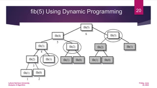
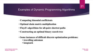
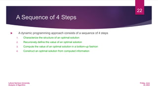
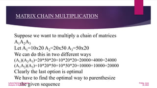
The document summarizes a lecture on dynamic programming and matrix chain multiplication. It discusses dynamic programming as a technique for solving optimization problems by breaking them down into overlapping subproblems and storing solutions. It then provides an example of using dynamic programming to find the most efficient way to multiply a chain of matrices by considering all possible parenthesizations and choosing the one with the lowest operation count. A 4-step process for dynamic programming problems is outlined.


![MATRIX MULTIPLICATION
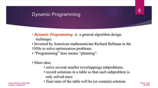
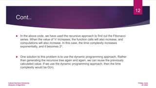
MATRIX MULTIPLY(A, B)
1. if columns[A]rows[B]
2. then error “incompatible dimension”
3. else
4. for i1 to rows[A]
5. do for j1 to columns[B]
6. do C[i,j] 0
7. for k1 to columns[A]
8. do C[i,j] C[i,j]+A[i,k]. B[k,j]
9. return C
Friday, June
24, 2022
Lahore Garrison University
Analysis of Algorithm](https://image.slidesharecdn.com/week9lec15-220624180522-c2800582/85/week-9-lec-15-pptx-23-320.jpg)
![MATRIX MULTIPLICATION
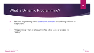
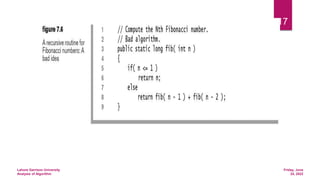
• Two matrices can only be multiplied if
columns[A] = rows [B]
• If order of A is p x q & order of B is q x r
then order of C will be p x r
• Time required to computer the product of two
matrices is p x q x r
Friday, June
24, 2022
Lahore Garrison University
Analysis of Algorithm](https://image.slidesharecdn.com/week9lec15-220624180522-c2800582/85/week-9-lec-15-pptx-24-320.jpg)
![August
2014
Amjad Ali
28
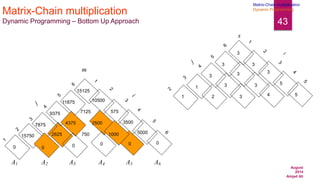
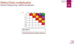
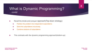
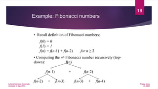
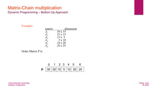
Matrix-Chain multiplication
Dynamic Programming – Bottom Up Approach
30 35 15 5 10 20 25
0 1 2 3 4 5 6
P
for l←2 to n
do for i←1 to n-l+1
do j←i+l-1
m[1,2]
m[2,3]
m[3,4]
m[4,5]
m[5,6]
1
2
3
4
6
5
1 2 3 4 5 6
1
2
3
4
6
5
1 2 3 4 5 6
m
S
0
0
0
0
0
0
l = 2
Matrix-Chain multiplication
Dynamic Programming](https://image.slidesharecdn.com/week9lec15-220624180522-c2800582/85/week-9-lec-15-pptx-28-320.jpg)
![29
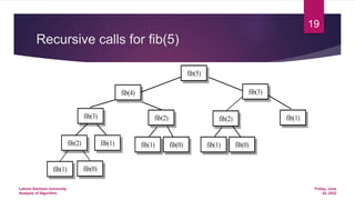
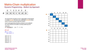
Matrix-Chain multiplication
Dynamic Programming – Bottom Up Approach
30 35 15 5 10 20 25
0 1 2 3 4 5 6
P
for l←2 to n
do for i←1 to n-l+1
do j←i+l-1
m[i, j] = min { m[i, k] +m[k+1, j] + pi-1 pk pj}
i ≤ k < j
m[1, 2] = min { m[1, 1] +m[2, 2] + p0 p1 p2}
1 ≤ k < 2
m[1, 2] = min { 0 + 0 + 30x35x15}
= min ( 15750 ) = 15750
m[2, 3] = min { m[2, 2] + m[3, 3] + p1 p2 p3}
2 ≤ k < 3
m[2, 3] = min { 0 + 0 + 35x15x5}
= min ( 2625 ) = 2625
1
2
3
4
6
5
1 2 3 4 5 6
1
2
3
4
6
5
1 2 3 4 5 6
m
S
0
0
0
0
0
0
15750
2625
1
2
l = 2
Matrix-Chain multiplication
Dynamic Programming](https://image.slidesharecdn.com/week9lec15-220624180522-c2800582/85/week-9-lec-15-pptx-29-320.jpg)
![30
Matrix-Chain multiplication
Dynamic Programming – Bottom Up Approach
30 35 15 5 10 20 25
0 1 2 3 4 5 6
P
for l←2 to n
do for i←1 to n-l+1
do j←i+l-1
m[3, 4] = min { m[3, 3] +m[4, 4] + p2 p3 p4}
3 ≤ k < 4
m[3, 4] = min { 0 + 0 + 15x5x10}
= min ( 750 ) = 750
m[4, 5] = min { m[4, 4] + m[5, 5] + p3 p4 p5}
4 ≤ k < 5
m[4, 5] = min { 0 + 0 + 5x10x20}
= min ( 1000 ) = 1000
m[5, 6] = min { m[5, 5] + m[6, 6] + p4 p5 p6}
5 ≤ k < 6
m[5, 6] = min { 0 + 0 + 10x20x25}
= min ( 5000 ) = 5000
1
2
3
4
6
5
1 2 3 4 5 6
1
2
3
4
6
5
1 2 3 4 5 6
m
S
0
0
0
0
0
0
15750
2625
1
2
750
3
1000
4
5000
5
l = 2
Matrix-Chain multiplication
Dynamic Programming](https://image.slidesharecdn.com/week9lec15-220624180522-c2800582/85/week-9-lec-15-pptx-30-320.jpg)
![August
2014
Amjad Ali
31
Matrix-Chain multiplication
Dynamic Programming – Bottom Up Approach
30 35 15 5 10 20 25
0 1 2 3 4 5 6
P
for l←2 to n
do for i←1 to n-l+1
do j←i+l-1
m[1, 3]
m[2, 4]
m[3, 5]
m[4, 6]
1
2
3
4
6
5
1 2 3 4 5 6
1
2
3
4
6
5
1 2 3 4 5 6
m
S
0
0
0
0
0
0
15750
2625
1
2
750
3
1000
4
5000
5
l = 3
Matrix-Chain multiplication
Dynamic Programming](https://image.slidesharecdn.com/week9lec15-220624180522-c2800582/85/week-9-lec-15-pptx-31-320.jpg)
![August
2014
Amjad Ali
32
Matrix-Chain multiplication
Dynamic Programming – Bottom Up Approach
30 35 15 5 10 20 25
0 1 2 3 4 5 6
P
for l←2 to n
do for i←1 to n-l+1
do j←i+l-1
m[1, 3]=min { m[1, 1] +m[2, 3] + p0 p1 p3 ,
1 ≤ k < 3 m[1, 2] +m[3, 3] + p0 p2 p3 }
m[1, 3] = min { 0 + 2625 + 30x35x5 ,
15750 + 0 +30x15x5 }
= min ( 7875 , 18000 ) = 7875
m[2, 4] = min { m[2, 2] + m[3, 4] + p1 p2 p4 ,
2 ≤ k < 4 m [2, 3]+m[4, 4] + p1 p3 p4 }
m[2, 4] = min { 0 + 750 + 35x15x10 ,
2625 + 0 + 35x5x10}
= min ( 6000, 4375) = 4375
1
2
3
4
6
5
1 2 3 4 5 6
1
2
3
4
6
5
1 2 3 4 5 6
m
S
0
0
0
0
0
0
15750
2625
1
2
750
3
1000
4
5000
5
7875
1
4375
3
l = 3
Matrix-Chain multiplication
Dynamic Programming](https://image.slidesharecdn.com/week9lec15-220624180522-c2800582/85/week-9-lec-15-pptx-32-320.jpg)
![August
2014
Amjad Ali
33
Matrix-Chain multiplication
Dynamic Programming – Bottom Up Approach
30 35 15 5 10 20 25
0 1 2 3 4 5 6
P
for l←2 to n
do for i←1 to n-l+1
do j←i+l-1
m[3, 5]=min { m[3, 3] +m[4, 5] + p2 p3 p5 ,
3 ≤ k < 5 m[3, 4] +m[5, 5] + p2 p4 p5 }
m[3, 5] = min { 0 + 1000 + 15x5x20 ,
750 + 0 +15x10x20 }
= min ( 2500 , 3750 ) = 2500
m[4, 6] = min { m[4, 4] + m[5, 6] + p3 p4 p6 ,
4 ≤ k < 6 m [4, 5]+m[6, 6] + p3 p5 p6 }
m[4, 6] = min { 0 + 5000 + 5x10x25 ,
1000 + 0 + 5x20x25}
= min ( 6250, 3500) = 3500
1
2
3
4
6
5
1 2 3 4 5 6
1
2
3
4
6
5
1 2 3 4 5 6
m
S
0
0
0
0
0
0
15750
2625
1
2
750
3
1000
4
5000
5
7875
1
4375
3
2500
3
3500
5
l = 3
Matrix-Chain multiplication
Dynamic Programming](https://image.slidesharecdn.com/week9lec15-220624180522-c2800582/85/week-9-lec-15-pptx-33-320.jpg)
![August
2014
Amjad Ali
34
Matrix-Chain multiplication
Dynamic Programming – Bottom Up Approach
30 35 15 5 10 20 25
0 1 2 3 4 5 6
P
m[1, 4]
m[2, 5]
m[3, 6]
1
2
3
4
6
5
1 2 3 4 5 6
1
2
3
4
6
5
1 2 3 4 5 6
m
S
0
0
0
0
0
0
15750
2625
1
2
750
3
1000
4
5000
5
7875
1
4375
3
2500
3
3500
5
l = 4
Matrix-Chain multiplication
Dynamic Programming](https://image.slidesharecdn.com/week9lec15-220624180522-c2800582/85/week-9-lec-15-pptx-34-320.jpg)
![August
2014
Amjad Ali
35
Matrix-Chain multiplication
Dynamic Programming – Bottom Up Approach
30 35 15 5 10 20 25
0 1 2 3 4 5 6
P
m[1, 4]=min { m[1, 1] + m[2, 4] + p0 p1 p4 ,
1 ≤ k < 4 m[1, 2] + m[3, 4] + p0 p2 p4 ,
m[1,3] + m[4,4] + p0 p3 p4 }
m[1, 4]=min { 0 + 4375 + 30x35x10 ,
15750 + 750 + 30x15x10
7875 + 0 + 30x5x10 }
m[1, 4]=min { 14875 , 21000 , 9375} = 9375
1
2
3
4
6
5
1 2 3 4 5 6
1
2
3
4
6
5
1 2 3 4 5 6
m
S
0
0
0
0
0
0
15750
2625
1
2
750
3
1000
4
5000
5
7875
1
4375
3
2500
3
3500
5
9375
3
l = 4
Matrix-Chain multiplication
Dynamic Programming](https://image.slidesharecdn.com/week9lec15-220624180522-c2800582/85/week-9-lec-15-pptx-35-320.jpg)
![August
2014
Amjad Ali
36
Matrix-Chain multiplication
Dynamic Programming – Bottom Up Approach
30 35 15 5 10 20 25
0 1 2 3 4 5 6
P
m[2, 5]=min { m[2, 2] + m[3, 5] + p1 p2 p5 ,
2 ≤ k < 5 m[2, 3] + m[4, 5] + p1 p3 p5 ,
m[2,4] + m[5,5] + p1 p4 p5 }
m[2, 5]=min { 0 + 2500 + 35x15x20 ,
2625+ 1000 + 35x5x20 ,
4375 + 0 + 35x10x20}
m[2, 5]=min { 13000 , 7125 , 11375} = 7125
1
2
3
4
6
5
1 2 3 4 5 6
1
2
3
4
6
5
1 2 3 4 5 6
m
S
0
0
0
0
0
0
15750
2625
1
2
750
3
1000
4
5000
5
7875
1
4375
3
2500
3
3500
5
9375
7125
3
3
l = 4
Matrix-Chain multiplication
Dynamic Programming](https://image.slidesharecdn.com/week9lec15-220624180522-c2800582/85/week-9-lec-15-pptx-36-320.jpg)
![August
2014
Amjad Ali
37
Matrix-Chain multiplication
Dynamic Programming – Bottom Up Approach
30 35 15 5 10 20 25
0 1 2 3 4 5 6
P
m[3, 6]=min { m[3, 3] + m[4, 6] + p2 p3 p6 ,
3 ≤ k < 6 m[3, 4] + m[5, 6] + p2 p4 p6 ,
m[3,5] + m[6,6] + p2 p5 p6 }
m[3, 6]=min { 0 + 3500 + 15x5x25 ,
750+ 5000 + 15x10x25 ,
2500 + 0 + 15x20x25}
m[3, 6]=min { 5375 , 9500 , 10000} = 5375
1
2
3
4
6
5
1 2 3 4 5 6
1
2
3
4
6
5
1 2 3 4 5 6
m
S
0
0
0
0
0
0
15750
2625
1
2
750
3
1000
4
5000
5
7875
1
4375
3
2500
3
3500
5
9375
5375
7125
3
3
3
l = 4
Matrix-Chain multiplication
Dynamic Programming](https://image.slidesharecdn.com/week9lec15-220624180522-c2800582/85/week-9-lec-15-pptx-37-320.jpg)
![August
2014
Amjad Ali
38
Matrix-Chain multiplication
Dynamic Programming – Bottom Up Approach
30 35 15 5 10 20 25
0 1 2 3 4 5 6
P
m[1, 5]
m[2, 6]
1
2
3
4
6
5
1 2 3 4 5 6
1
2
3
4
6
5
1 2 3 4 5 6
m
S
0
0
0
0
0
0
15750
2625
1
2
750
3
1000
4
5000
5
7875
1
4375
3
2500
3
3500
5
9375
5375
7175
3
3
3
l = 5
Matrix-Chain multiplication
Dynamic Programming](https://image.slidesharecdn.com/week9lec15-220624180522-c2800582/85/week-9-lec-15-pptx-38-320.jpg)
![August
2014
Amjad Ali
39
Matrix-Chain multiplication
Dynamic Programming – Bottom Up Approach
30 35 15 5 10 20 25
0 1 2 3 4 5 6
P
m[1, 5]=min { m[1, 1] + m[2, 5] + p0 p1 p5 ,
1 ≤ k < 5 m[1, 2] + m[3, 5] + p0 p2 p5 ,
m[1,3] + m[4,5] + p0 p3 p5 ,
m[1, 4] + m[5, 5] + p0 p4 p5 }
m[1, 5]=min { 0 + 7175 + 30x35x20 ,
15750 + 2500 + 30x15x20 ,
7875 + 1000 + 30x5x20 ,
9375 + 0 + 30x10x20}
m[1, 5]=min { 28175 , 27250 , 11875 , 15375}
= 11875
1
2
3
4
6
5
1 2 3 4 5 6
1
2
3
4
6
5
1 2 3 4 5 6
m
S
0
0
0
0
0
0
15750
2625
1
2
750
3
1000
4
5000
5
7875
1
4375
3
2500
3
3500
5
9375
5375
7175
3
3
3
l = 5
11875
3
Matrix-Chain multiplication
Dynamic Programming](https://image.slidesharecdn.com/week9lec15-220624180522-c2800582/85/week-9-lec-15-pptx-39-320.jpg)
![August
2014
Amjad Ali
40
Matrix-Chain multiplication
Dynamic Programming – Bottom Up Approach
30 35 15 5 10 20 25
0 1 2 3 4 5 6
P
m[2, 6]=min { m[2, 2] + m[3, 6] + p1 p2 p6 ,
2 ≤ k < 6 m[2, 3] + m[4, 6] + p1 p3 p6 ,
m[2,4] + m[5,6] + p1 p4 p6 ,
m[2, 5] + m[6, 6] + p1 p5 p6 }
m[2, 6]=min { 0 + 5375 + 35x15x25 ,
2625+ 3500 + 35x5x25 ,
4375 + 5000 + 35x10x25 ,
5725 + 0 + 35x20x25}
m[2, 6]=min { 18500 , 10500 , 18125 , 23225}
= 10500
1
2
3
4
6
5
1 2 3 4 5 6
1
2
3
4
6
5
1 2 3 4 5 6
m
S
0
0
0
0
0
0
15750
2625
1
2
750
3
1000
4
5000
5
7875
1
4375
3
2500
3
3500
5
9375
5375
5725
3
3
3
l = 5
3
10500
3
11875
Matrix-Chain multiplication
Dynamic Programming](https://image.slidesharecdn.com/week9lec15-220624180522-c2800582/85/week-9-lec-15-pptx-40-320.jpg)
![August
2014
Amjad Ali
41
Matrix-Chain multiplication
Dynamic Programming – Bottom Up Approach
30 35 15 5 10 20 25
0 1 2 3 4 5 6
P
m[1, 6]
1
2
3
4
6
5
1 2 3 4 5 6
1
2
3
4
6
5
1 2 3 4 5 6
m
S
0
0
0
0
0
0
15750
2625
1
2
750
3
1000
4
5000
5
7875
1
4375
3
2500
3
3500
5
9375
5375
5725
3
3
3
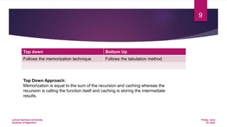
l = 6
3
10500
3
11875
Matrix-Chain multiplication
Dynamic Programming](https://image.slidesharecdn.com/week9lec15-220624180522-c2800582/85/week-9-lec-15-pptx-41-320.jpg)
![August
2014
Amjad Ali
42
Matrix-Chain multiplication
Dynamic Programming – Bottom Up Approach
30 35 15 5 10 20 25
0 1 2 3 4 5 6
P
m[1, 6]=min { m[1, 1] + m[2, 6] + p0 p1 p6 ,
1 ≤ k < 6 m[1, 2] + m[3, 6] + p0 p2 p6 ,
m[1,3] + m[4,6] + p0 p3 p6 ,
m[1, 4] + m[5, 6] + p0 p4 p6 ,
m[1, 5] + m[6, 6] + p0 p5 p6 }
m[1, 6]=min { 0 + 10500 + 30x35x25,
15750+ 5375 + 30x15x25 ,
7875 + 3500 + 30x5x25 ,
9375+ 5000 + 30x10x25 ,
11875+ 0 + 30x20x25}
m[1, 6]=min { 36750 , 32375 , 15125 , 26875}
= 15125
1
2
3
4
6
5
1 2 3 4 5 6
1
2
3
4
6
5
1 2 3 4 5 6
m
S
0
0
0
0
0
0
15750
2625
1
2
750
3
1000
4
5000
5
7875
1
4375
3
2500
3
3500
5
9375
5375
5725
3
3
3
l = 6
3
10500
3
11875
3
15125
Matrix-Chain multiplication
Dynamic Programming](https://image.slidesharecdn.com/week9lec15-220624180522-c2800582/85/week-9-lec-15-pptx-42-320.jpg)