DATA STRUCTURE.pdf

DATA STRUCTURES
LECTURE NOTES
Dr.K VENKATA NAGENDRA
Mr.G.RAJESH

DATA STRUCTURES(18CS202)
OBJECTIVES:
The course should enable the students to :
1. Demonstrate familiarity with major algorithms and data structures.
2. Choose the appropriate data structure and algorithm design method for a specified
application.
3. Determine which algorithm or data structure to use in different scenarios.
4. To improve the logical ability.
UNIT-I INTRODUCTION TO ALGORITHMS AND DATA
STRUCTURES
Classes:12
Algorithms: Definition, Properties, Performance Analysis-Space Complexity, Time Complexity,
Asymptotic Notations.Data structures: Introduction, Data Structures types, DS Operations.
UNIT-II STACKS AND QUEUES Classes:12
Stacks: Introduction, Stack Operations, Applications: Infix to Postfix Conversion, Evaluation of
Postfix Expression.ueues: Introduction, Operations on queues, Circular queues, Priority queues.
UNIT-III LINKED LISTS AND APPLICATIONS Classes:12
Linked lists: Introduction, Singly linked lists, Circular linked lists, Doubly linked lists, Multiply
linked lists, Applications: Polynomial Representation.Implementation of Stack and Queue using
linked list.
UNIT-IV SORTING AND SEARCHING Classes:12
Sorting: Introduction, Selection sort, Bubble sort, Insertion sort, Merge sort, Quick sort, Heap
Sort.Searching: Introduction, Linear search, Binary search, Fibonacci search.
UNIT-V TREES AND BINARY TREES Classes:12
Trees: Introduction, Definition and basic terminologies, Representation of trees.
Binary Trees: Basic Terminologies and Types, Binary Tree Traversals, Binary Search Trees.
Text Books:
1. G.A.V PAI, Data Structures and Algorithms, Concepts, Techniques and Applications,
Volume1, 1stEdition, Tata McGraw-Hill, 2008.
2. Richard F. Gilberg& Behrouz A. Forouzan, Data Structures, Pseudo code Approach with
C, 2ndEdition, Cengage Learning India Edition, 2007.
Reference Books:
1. Langsam,M. J. Augenstein, A. M. Tanenbaum, Datastructures using C and C++, 2nd
Edition, PHI Education, 2008.
2. Sartaj Sahni, Ellis Horowitz, Fundamentals of at Structures in C, 2nd Edition,
Orientblackswan, 2010.
Web References:
1. https://www.geeksforgeeks.org/data-structures/
2. https://www.programiz.com/dsa
3. https://www.w3schools.in/data-structures-tutorial/intro/
Outcomes:
At the end of the course students able to
1. Apply Concepts of Stacks, Queues, Linked Lists.
2. Develop Programs for Searching and Sorting, Trees.
3. Interpret concepts of trees.
4. Develop programs for Sorting and Searching.

1
UNIT-I
INTRODUCTION TO ALGORITHMS AND DATA STRUCTURES
Definition: - An algorithm is a Step By Step process to solve a problem, where each step
indicates an intermediate task. Algorithm contains finite number of steps that leads to the
solution of the problem.
Properties /Characteristics of an Algorithm:-
Algorithm has the following basic properties
 Input-Output:- Algorithm takes ‘0’ or more input and produces the required output.
This is the basic characteristic of an algorithm.
 Finiteness:- An algorithm must terminate in countable number of steps.
 Definiteness: Each step of an algorithm must be stated clearly and unambiguously.
 Effectiveness: Each and every step in an algorithm can be converted in to
programming language statement.
 Generality: Algorithm is generalized one. It works on all set of inputs and provides
the required output. In other words it is not restricted to a single input value.
Categories of Algorithm:
Based on the different types of steps in an Algorithm, it can be divided into three
categories, namely
 Sequence
 Selection and
 Iteration
Sequence: The steps described in an algorithm are performed successively one by one
without skipping any step. The sequence of steps defined in an algorithm should be simple
and easy to understand. Each instruction of such an algorithm is executed, because no
selection procedure or conditional branching exists in a sequence algorithm.
Example:
// adding two numbers
Step 1: start
Step 2: read a,b
Step 3: Sum=a+b
Step 4: write Sum
Step 5: stop
Selection: The sequence type of algorithms are not sufficient to solve the problems, which
involves decision and conditions. In order to solve the problem which involve decision
making or option selection, we go for Selection type of algorithm. The general format of
Selection type of statement is as shown below:
if(condition)
Statement-1;
else
Statement-2;
The above syntax specifies that if the condition is true, statement-1 will be executed
otherwise statement-2 will be executed. In case the operation is unsuccessful. Then
sequence of algorithm should be changed/ corrected in such a way that the system will re-
execute until the operation is successful.

2
Iteration: Iteration type algorithms are used in solving the problems which involves
repetition of statement. In this type of algorithms, a particular number of statements are
repeated ‘n’ no. of times.
Example1:
Step 1 : start
Step 2 : read n
Step 3 : repeat step 4 until n>0
Step 4 : (a) r=n mod 10
(b) s=s+r
(c) n=n/10
Step 5 : write s
Step 6 : stop
Performance Analysis an Algorithm:
The Efficiency of an Algorithm can be measured by the following metrics.
i. Time Complexity and
ii. Space Complexity.
i.Time Complexity:
The amount of time required for an algorithm to complete its execution is its time
complexity. An algorithm is said to be efficient if it takes the minimum (reasonable) amount
of time to complete its execution.
ii. Space Complexity:
The amount of space occupied by an algorithm is known as Space Complexity. An algorithm
is said to be efficient if it occupies less space and required the minimum amount of time to
complete its execution.
1.Write an algorithm for roots of a Quadratic Equation?
// Roots of a quadratic Equation
Step 1 : start
Step 2 : read a,b,c
Step 3 : if (a= 0) then step 4 else step 5
Step 4 : Write “ Given equation is a linear equation “
Step 5 : d=(b * b) _ (4 *a *c)
Step 6 : if ( d>0) then step 7 else step8
Step 7 : Write “ Roots are real and Distinct”
Step 8: if(d=0) then step 9 else step 10
Step 9: Write “Roots are real and equal”
Step 10: Write “ Roots are Imaginary”
Step 11: stop

3
2. Write an algorithm to find the largest among three different numbers entered by user
Step 1: Start
Step 2: Declare variables a,b and c.
Step 3: Read variables a,b and c.
Step 4: If a>b
If a>c
Display a is the largest number.
Else
Display c is the largest number.
Else
If b>c
Display b is the largest number.
Else
Display c is the greatest number.
Step 5: Stop
3.Write an algorithm to find the factorial of a number entered by user.
Step 1: Start
Step 2: Declare variables n,factorial and i.
Step 3: Initialize variables
factorial←1
i←1
Step 4: Read value of n
Step 5: Repeat the steps until i=n
5.1: factorial←factorial*i
5.2: i←i+1
Step 6: Display factorial
Step 7: Stop
4.Write an algorithm to find the Simple Interest for given Time and Rate of Interest .
Step 1: Start
Step 2: Read P,R,S,T.
Step 3: Calculate S=(PTR)/100
Step 4: Print S
Step 5: Stop
ASYMPTOTIC NOTATIONS
Asymptotic analysis of an algorithm refers to defining the mathematical
boundation/framing of its run-time performance. Using asymptotic analysis, we can very
well conclude the best case, average case, and worst case scenario of an algorithm.
Asymptotic analysis is input bound i.e., if there's no input to the algorithm, it is concluded
to work in a constant time. Other than the "input" all other factors are considered
constant.
Asymptotic analysis refers to computing the running time of any operation in mathematical
units of computation. For example, the running time of one operation is computed as f(n)
and may be for another operation it is computed as g(n2
). This means the first operation
running time will increase linearly with the increase in n and the running time of the
second operation will increase exponentially when n increases. Similarly, the running time
of both operations will be nearly the same if n is significantly small.

4
The time required by an algorithm falls under three types −
 Best Case − Minimum time required for program execution.
 Average Case − Average time required for program execution.
 Worst Case − Maximum time required for program execution.
Asymptotic Notations
Following are the commonly used asymptotic notations to calculate the running time
complexity of an algorithm.
 Ο Notation
 Ω Notation
 θ Notation
Big Oh Notation, Ο
The notation Ο(n) is the formal way to express the upper bound of an algorithm's running
time. It measures the worst case time complexity or the longest amount of time an
algorithm can possibly take to complete.
For example, for a function f(n)
Ο(f(n)) = { g(n) : there exists c > 0 and n0 such that f(n) ≤ c.g(n) for all n > n0. }
Omega Notation, Ω
The notation Ω(n) is the formal way to express the lower bound of an algorithm's running
time. It measures the best case time complexity or the best amount of time an algorithm
can possibly take to complete.
For example, for a function f(n)
Ω(f(n)) ≥ { g(n) : there exists c > 0 and n0 such that g(n) ≤ c.f(n) for all n > n0. }
Theta Notation, θ
The notation θ(n) is the formal way to express both the lower bound and the upper bound
of an algorithm's running time. It is represented as follows −

5
θ(f(n)) = { g(n) if and only if g(n) = Ο(f(n)) and g(n) = Ω(f(n)) for all n > n0. }
DATA STRUCTURES
Data may be organized in many different ways logical or mathematical model of a program
particularly organization of data. This organized data is called “Data Structure”.
Or
The organized collection of data is called a ‘Data Structure’.
Data Structure involves two complementary goals. The first goal is to identify and develop
useful, mathematical entities and operations and to determine what class of problems can
be solved by using these entities and operations. The second goal is to determine
representation for those abstract entities to implement abstract operations on this concrete
representation.
Primitive Data structures are directly supported by the language ie; any operation is directly
performed in these data items.
Ex: integer, Character, Real numbers etc.
Non-primitive data types are not defined by the programming language, but are instead
created by the programmer.
Data Structure=Organized data +Allowed operations

6
Linear data structures organize their data elements in a linear fashion, where data
elements are attached one after the other. Linear data structures are very easy to
implement, since the memory of the computer is also organized in a linear fashion. Some
commonly used linear data structures are arrays, linked lists, stacks and queues.
In nonlinear data structures, data elements are not organized in a sequential
fashion. Data structures like multidimensional arrays, trees, graphs, tables and sets are
some examples of widely used nonlinear data structures.
Operations on the Data Structures:
Following operations can be performed on the data structures:
1. Traversing
2. Searching
3. Inserting
4. Deleting
5. Sorting
6. Merging
1. Traversing- It is used to access each data item exactly once so that it can be processed.
2. Searching- It is used to find out the location of the data item if it exists in the given
collection of data items.
3. Inserting- It is used to add a new data item in the given collection of data items.
4. Deleting- It is used to delete an existing data item from the given collection of data items.
5. Sorting- It is used to arrange the data items in some order i.e. in ascending or descending
order in case of numerical data and in dictionary order in case of alphanumeric data.
6. Merging- It is used to combine the data items of two sorted files into single file in the
sorted form.

7
UNIT-II
STACKS AND QUEUES
STACKS
A Stack is linear data structure. A stack is a list of elements in which an element may be
inserted or deleted only at one end, called the top of the stack. Stack principle is LIFO (last
in, first out). Which element inserted last on to the stack that element deleted first from the
stack.
As the items can be added or removed only from the top i.e. the last item to be added to a
stack is the first item to be removed.
Real life examples of stacks are:
Operations on stack:
The two basic operations associated with stacks are:
1. Push
2. Pop
While performing push and pop operations the following test must be conducted on the
stack.
a) Stack is empty or not b) stack is full or not
1. Push: Push operation is used to add new elements in to the stack. At the time of addition
first check the stack is full or not. If the stack is full it generates an error message "stack
overflow".
2. Pop: Pop operation is used to delete elements from the stack. At the time of deletion first
check the stack is empty or not. If the stack is empty it generates an error message "stack
underflow".
All insertions and deletions take place at the same end, so the last element added to
the stack will be the first element removed from the stack. When a stack is created, the
stack base remains fixed while the stack top changes as elements are added and removed.
The most accessible element is the top and the least accessible element is the bottom of the
stack.

8
Representation of Stack (or) Implementation of stack:
The stack should be represented in two ways:
1. Stack using array
2. Stack using linked list
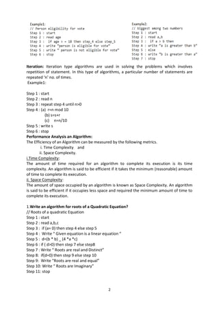
1. Stack using array:
Let us consider a stack with 6 elements capacity. This is called as the size of the stack. The
number of elements to be added should not exceed the maximum size of the stack. If we
attempt to add new element beyond the maximum size, we will encounter a stack overflow
condition. Similarly, you cannot remove elements beyond the base of the stack. If such is
the case, we will reach a stack underflow condition.
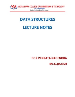
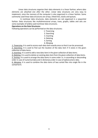
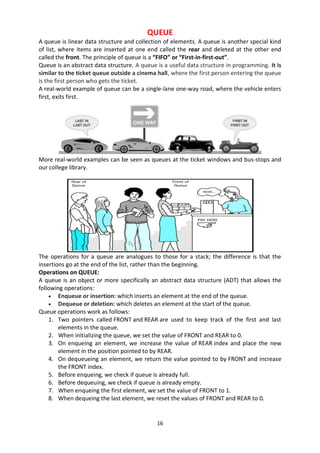
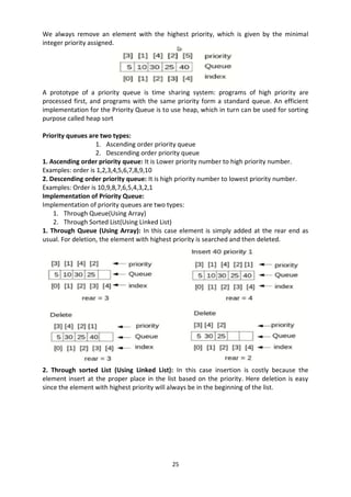
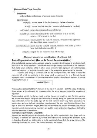
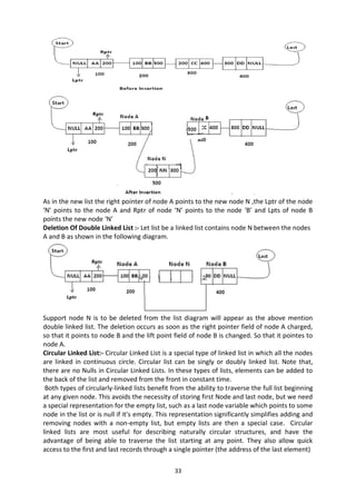
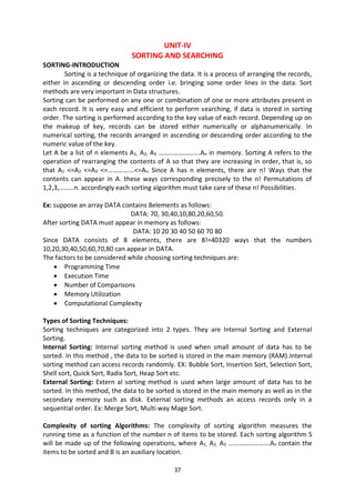
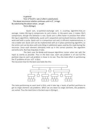
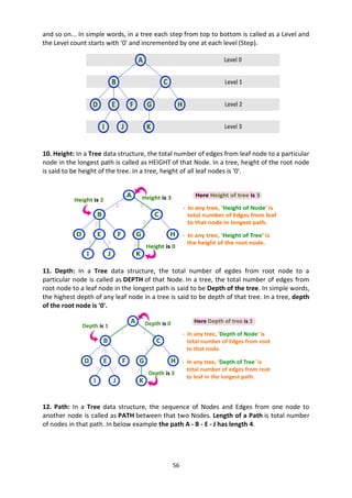
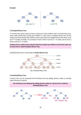
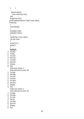
1.push():When an element is added to a stack, the operation is performed by push(). Below
Figure shows the creation of a stack and addition of elements using push().
Initially top=-1, we can insert an element in to the stack, increment the top value i.e
top=top+1. We can insert an element in to the stack first check the condition is stack is full
or not. i.e top>=size-1. Otherwise add the element in to the stack.
void push()
{
int x;
if(top >= n-1)
{
printf("nnStack
Overflow..");
return;
}
else
{
printf("nnEnter data: ");
scanf("%d", &x);
stack[top] = x;
top = top + 1;
printf("nnData Pushed into
the stack");
}
}
Algorithm: Procedure for push():
Step 1: START
Step 2: if top>=size-1 then
Write “ Stack is Overflow”
Step 3: Otherwise
3.1: read data value ‘x’
3.2: top=top+1;
3.3: stack[top]=x;
Step 4: END

9
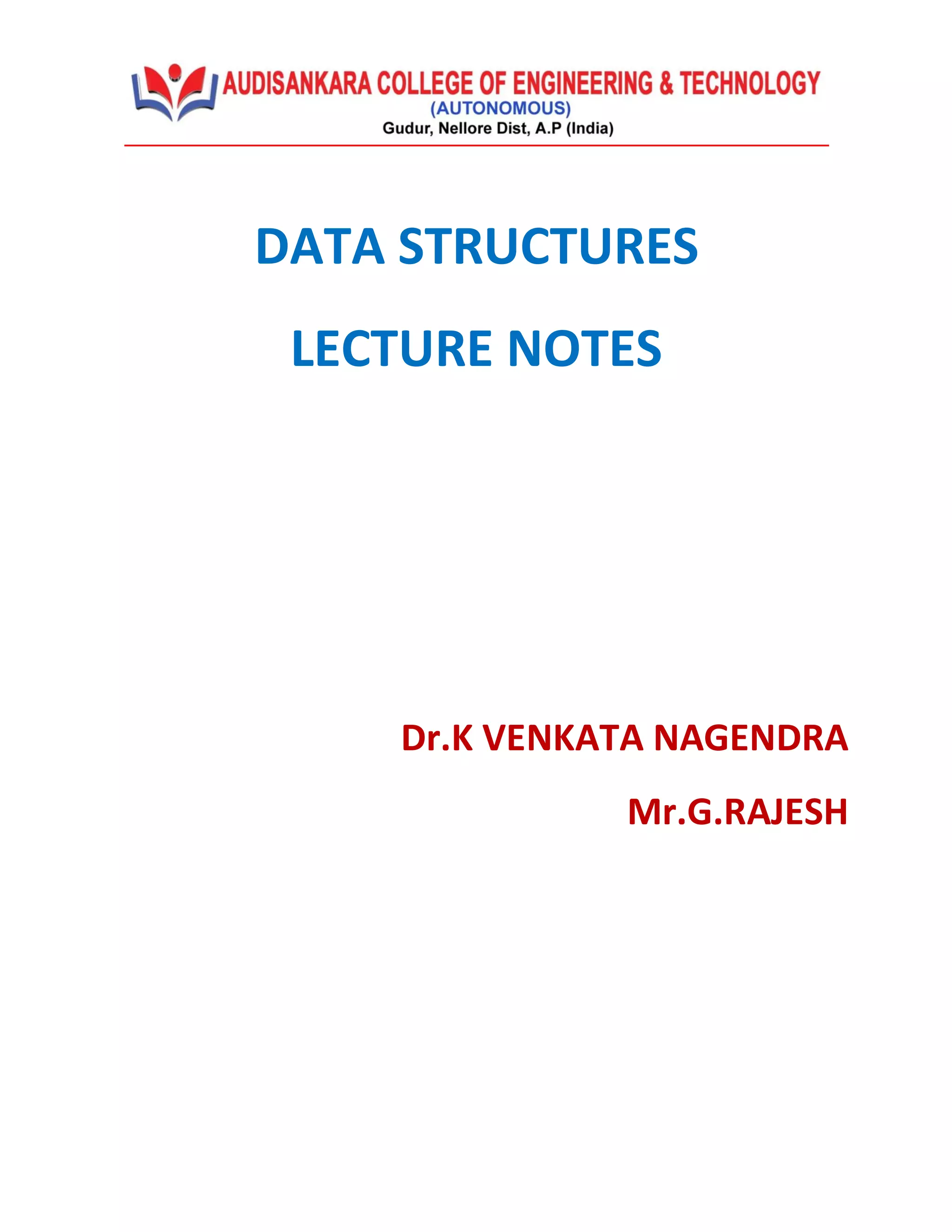
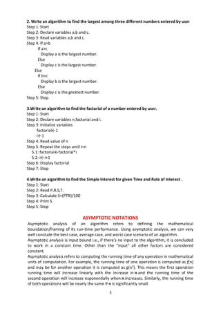
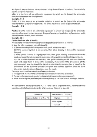
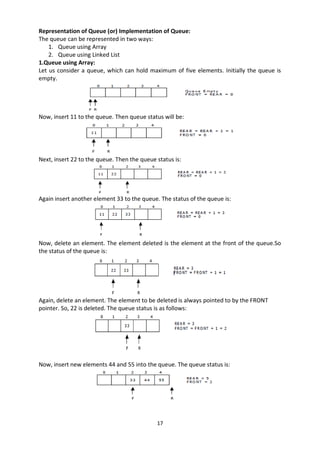
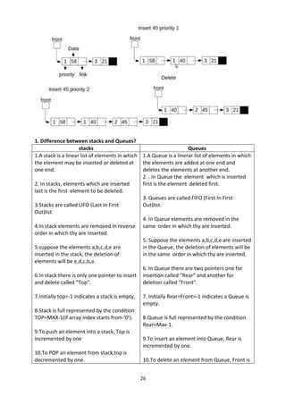
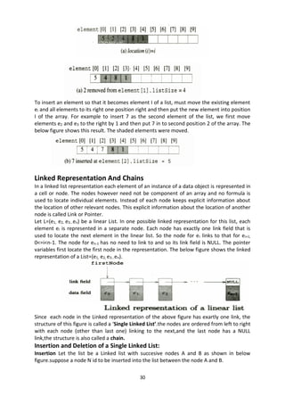
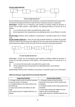
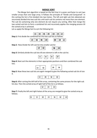
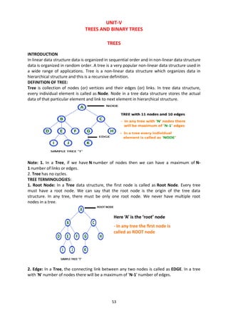
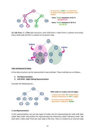
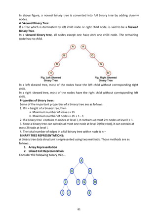
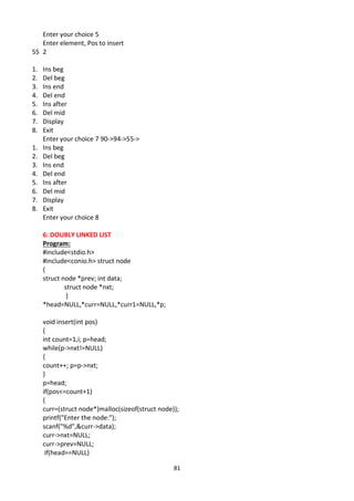
2.Pop(): When an element is taken off from the stack, the operation is performed by pop().
Below figure shows a stack initially with three elements and shows the deletion of elements
using pop().
We can insert an element from the stack, decrement the top value i.e top=top-1.
We can delete an element from the stack first check the condition is stack is empty or not.
i.e top==-1. Otherwise remove the element from the stack.
Void pop()
{
If(top==-1)
{
Printf(“Stack is Underflow”);
}
else
{
printf(“Delete data %d”,stack[top]);
top=top-1;
}
}
Algorithm: procedure pop():
Step 1: START
Step 2: if top==-1 then
Write “Stack is Underflow”
Step 3: otherwise
3.1: print “deleted element”
3.2: top=top-1;
Step 4: END
3.display(): This operation performed display the elements in the stack. We display the
element in the stack check the condition is stack is empty or not i.e top==-1.Otherwise
display the list of elements in the stack.

10
void display()
{
If(top==-1)
{
Printf(“Stack is Underflow”);
}
else
{
printf(“Display elements are:);
for(i=top;i>=0;i--)
printf(“%d”,stack[i]);
}
}
Algorithm: procedure pop():
Step 1: START
Step 2: if top==-1 then
Write “Stack is Underflow”
Step 3: otherwise
3.1: print “Display elements are”
3.2: for top to 0
Print ‘stack[i]’
Step 4: END
Source code for stack operations, using array:
#include<stdio.h>
#inlcude<conio.h>
int stack[100],choice,n,top,x,i;
void push(void);
void pop(void);
void display(void);
int main()
{
//clrscr();
top=-1;
printf("n Enter the size of STACK[MAX=100]:");
scanf("%d",&n);
printf("nt STACK OPERATIONS USING ARRAY");
printf("nt--------------------------------");
printf("nt 1.PUSHnt 2.POPnt 3.DISPLAYnt 4.EXIT");
do
{
printf("n Enter the Choice:");
scanf("%d",&choice);
switch(choice)
{
case 1:
{
push();
break;
}
case 2:
{
pop();
break;
}
case 3:
{

11
display();
break;
}
case 4:
{
printf("nt EXIT POINT ");
break;
}
default:
{
printf ("nt Please Enter a Valid Choice(1/2/3/4)");
}
}
}
while(choice!=4);
return 0;
}
void push()
{
if(top>=n-1)
{
printf("ntSTACK is over flow");
}
else
{
printf(" Enter a value to be pushed:");
scanf("%d",&x);
top++;
stack[top]=x;
}
}
void pop()
{
if(top<=-1)
{
printf("nt Stack is under flow");
}
else
{
printf("nt The popped elements is %d",stack[top]);
top--;
}
}
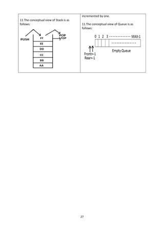
void display()
{
if(top>=0)
{

12
printf("n The elements in STACK n");
for(i=top; i>=0; i--)
printf("n%d",stack[i]);
printf("n Press Next Choice");
}
else
{
printf("n The STACK is empty");
}
}
2. Stack using Linked List:
We can represent a stack as a linked list. In a stack push and pop operations are performed
at one end called top. We can perform similar operations at one end of list using top
pointer. The linked stack looks as shown in figure.
Applications of stack:
1. Stack is used by compilers to check for balancing of parentheses, brackets and braces.
2. Stack is used to evaluate a postfix expression.
3. Stack is used to convert an infix expression into postfix/prefix form.
4. In recursion, all intermediate arguments and return values are stored on the processor’s
stack.
5. During a function call the return address and arguments are pushed onto a stack and on
return they are popped off.
Converting and evaluating Algebraic expressions:
An algebraic expression is a legal combination of operators and operands. Operand is the
quantity on which a mathematical operation is performed. Operand may be a variable like x,
y, z or a constant like 5, 4, 6 etc. Operator is a symbol which signifies a mathematical or
logical operation between the operands. Examples of familiar operators include +, -, *, /, ^
etc.

13
An algebraic expression can be represented using three different notations. They are infix,
postfix and prefix notations:
Infix: It is the form of an arithmetic expression in which we fix (place) the arithmetic
operator in between the two operands.
Example: A + B
Prefix: It is the form of an arithmetic notation in which we fix (place) the arithmetic
operator before (pre) its two operands. The prefix notation is called as polish notation.
Example: + A B
Postfix: It is the form of an arithmetic expression in which we fix (place) the arithmetic
operator after (post) its two operands. The postfix notation is called as suffix notation and is
also referred to reverse polish notation.
Example: A B +
Conversion from infix to postfix:
Procedure to convert from infix expression to postfix expression is as follows:
1. Scan the infix expression from left to right.
2. a) If the scanned symbol is left parenthesis, push it onto the stack.
b) If the scanned symbol is an operand, then place directly in the postfix expression
(output).
c) If the symbol scanned is a right parenthesis, then go on popping all the items from the
stack and place them in the postfix expression till we get the matching left parenthesis.
d) If the scanned symbol is an operator, then go on removing all the operators from the
stack and place them in the postfix expression, if and only if the precedence of the
operator which is on the top of the stack is greater than (or greater than or equal) to the
precedence of the scanned operator and push the scanned operator onto the stack
otherwise, push the scanned operator onto the stack.
The three important features of postfix expression are:
1. The operands maintain the same order as in the equivalent infix expression.
2. The parentheses are not needed to designate the expression unambiguously.
3. While evaluating the postfix expression the priority of the operators is no longer relevant.
We consider five binary operations: +, -, *, / and $ or ↑ (exponentiation). For these binary
operations, the following in the order of precedence (highest to lowest):

14
Evaluation of postfix expression:
The postfix expression is evaluated easily by the use of a stack.
1. When a number is seen, it is pushed onto the stack;
2. When an operator is seen, the operator is applied to the two numbers that are
popped from the stack and the result is pushed onto the stack.
3. When an expression is given in postfix notation, there is no need to know any
precedence rules; this is our obvious advantage.

16
QUEUE
A queue is linear data structure and collection of elements. A queue is another special kind
of list, where items are inserted at one end called the rear and deleted at the other end
called the front. The principle of queue is a “FIFO” or “First-in-first-out”.
Queue is an abstract data structure. A queue is a useful data structure in programming. It is
similar to the ticket queue outside a cinema hall, where the first person entering the queue
is the first person who gets the ticket.
A real-world example of queue can be a single-lane one-way road, where the vehicle enters
first, exits first.
More real-world examples can be seen as queues at the ticket windows and bus-stops and
our college library.
The operations for a queue are analogues to those for a stack; the difference is that the
insertions go at the end of the list, rather than the beginning.
Operations on QUEUE:
A queue is an object or more specifically an abstract data structure (ADT) that allows the
following operations:
 Enqueue or insertion: which inserts an element at the end of the queue.
 Dequeue or deletion: which deletes an element at the start of the queue.
Queue operations work as follows:
1. Two pointers called FRONT and REAR are used to keep track of the first and last
elements in the queue.
2. When initializing the queue, we set the value of FRONT and REAR to 0.
3. On enqueing an element, we increase the value of REAR index and place the new
element in the position pointed to by REAR.
4. On dequeueing an element, we return the value pointed to by FRONT and increase
the FRONT index.
5. Before enqueing, we check if queue is already full.
6. Before dequeuing, we check if queue is already empty.
7. When enqueing the first element, we set the value of FRONT to 1.
8. When dequeing the last element, we reset the values of FRONT and REAR to 0.

17
Representation of Queue (or) Implementation of Queue:
The queue can be represented in two ways:
1. Queue using Array
2. Queue using Linked List
1.Queue using Array:
Let us consider a queue, which can hold maximum of five elements. Initially the queue is
empty.
Now, insert 11 to the queue. Then queue status will be:
Next, insert 22 to the queue. Then the queue status is:
Again insert another element 33 to the queue. The status of the queue is:
Now, delete an element. The element deleted is the element at the front of the queue.So
the status of the queue is:
Again, delete an element. The element to be deleted is always pointed to by the FRONT
pointer. So, 22 is deleted. The queue status is as follows:
Now, insert new elements 44 and 55 into the queue. The queue status is:

18
Next insert another element, say 66 to the queue. We cannot insert 66 to the queue as the
rear crossed the maximum size of the queue (i.e., 5). There will be queue full signal. The
queue status is as follows:
Now it is not possible to insert an element 66 even though there are two vacant positions in
the linear queue. To overcome this problem the elements of the queue are to be shifted
towards the beginning of the queue so that it creates vacant position at the rear end. Then
the FRONT and REAR are to be adjusted properly. The element 66 can be inserted at the
rear end. After this operation, the queue status is as follows:
This difficulty can overcome if we treat queue position with index 0 as a position that comes
after position with index 4 i.e., we treat the queue as a circular queue.
Queue operations using array:
a.enqueue() or insertion():which inserts an element at the end of the queue.
void insertion()
{
if(rear==max)
printf("n Queue is Full");
else
{
printf("n Enter no %d:",j++);
scanf("%d",&queue[rear++]);
}
}
Algorithm: Procedure for insertion():
Step-1:START
Step-2: if rear==max then
Write ‘Queue is full’
Step-3: otherwise
3.1: read element ‘queue[rear]’
Step-4:STOP
b.dequeue() or deletion(): which deletes an element at the start of the queue.
void deletion()
{
if(front==rear)
{
printf("n Queue is empty");
}
else
{
printf("n Deleted Element is
%d",queue[front++]);
x++;
} }
Algorithm: procedure for deletion():
Step-1:START
Step-2: if front==rear then
Write’ Queue is empty’
Step-3: otherwise
3.1: print deleted element
Step-4:STOP

19
c.dispaly(): which displays an elements in the queue.
void deletion()
{
if(front==rear)
{
printf("n Queue is empty");
}
else
{
for(i=front; i<rear; i++)
{
printf("%d",queue[i]);
printf("n");
}
}
}
Algorithm: procedure for deletion():
Step-1:START
Step-2: if front==rear then
Write’ Queue is empty’
Step-3: otherwise
3.1: for i=front to rear then
3.2: print ‘queue[i]’
Step-4:STOP
2. Queue using Linked list:
We can represent a queue as a linked list. In a queue data is deleted from the front end and
inserted at the rear end. We can perform similar operations on the two ends of alist. We use
two pointers front and rear for our linked queue implementation.
The linked queue looks as shown in figure:
Applications of Queue:
1. It is used to schedule the jobs to be processed by the CPU.
2. When multiple users send print jobs to a printer, each printing job is kept in the printing
queue. Then the printer prints those jobs according to first in first out (FIFO) basis.
3. Breadth first search uses a queue data structure to find an element from a graph.

20
CIRCULAR QUEUE
A more efficient queue representation is obtained by regarding the array Q[MAX] as
circular. Any number of items could be placed on the queue. This implementation of a
queue is called a circular queue because it uses its storage array as if it were a circle instead
of a linear list.
There are two problems associated with linear queue. They are:
 Time consuming: linear time to be spent in shifting the elements to the beginning of
the queue.
 Signaling queue full: even if the queue is having vacant position.
For example, let us consider a linear queue status as follows:
Next insert another element, say 66 to the queue. We cannot insert 66 to the queue as the
rear crossed the maximum size of the queue (i.e., 5). There will be queue full signal. The
queue status is as follows:
This difficulty can be overcome if we treat queue position with index zero as a position that
comes after position with index four then we treat the queue as a circular queue.
In circular queue if we reach the end for inserting elements to it, it is possible to insert new
elements if the slots at the beginning of the circular queue are empty.
Representation of Circular Queue:
Let us consider a circular queue, which can hold maximum (MAX) of six elements. Initially
the queue is empty.
Now, insert 11 to the circular queue. Then circular queue status will be:

21
Insert new elements 22, 33, 44 and 55 into the circular queue. The circular queue status is:
Now, delete an element. The element deleted is the element at the front of the circular
queue. So, 11 is deleted. The circular queue status is as follows:
Again, delete an element. The element to be deleted is always pointed to by the FRONT
pointer. So, 22 is deleted. The circular queue status is as follows:
Again, insert another element 66 to the circular queue. The status of the circular queue is:

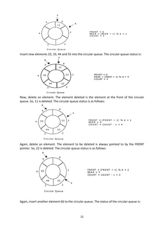
22
Now, insert new elements 77 and 88 into the circular queue. The circular queue status is:
Now, if we insert an element to the circular queue, as COUNT = MAX we cannot add the
element to circular queue. So, the circular queue is full.
Operations on Circular queue:
a.enqueue() or insertion():This function is used to insert an element into the circular queue.
In a circular queue, the new element is always inserted at Rear position.
void insertCQ()
{
int data;
if(count ==MAX)
{
printf("n Circular Queue is Full");
}
else
{
printf("n Enter data: ");
scanf("%d", &data);
CQ[rear] = data;
rear = (rear + 1) % MAX;
count ++;
printf("n Data Inserted in the Circular
Queue ");
}
}
Algorithm: procedure of insertCQ():
Step-1:START
Step-2: if count==MAX then
Write “Circular queue is full”
Step-3:otherwise
3.1: read the data element
3.2: CQ[rear]=data
3.3: rear=(rear+1)%MAX
3.4: count=count+1
Step-4:STOP

23
b.dequeue() or deletion():This function is used to delete an element from the circular
queue. In a circular queue, the element is always deleted from front position.
void deleteCQ()
{
if(count ==0)
{
printf("nnCircular Queue is Empty..");
}
else
{
printf("n Deleted element from Circular
Queue is %d ", CQ[front]);
front = (front + 1) % MAX;
count --;
}
}
Algorithm: procedure of deleteCQ():
Step-1:START
Step-2: if count==0 then
Write “Circular queue is empty”
Step-3:otherwise
3.1: print the deleted element
3.2: front=(front+1)%MAX
3.3: count=count-1
Step-4:STOP
c.dispaly():This function is used to display the list of elements in the circular queue.
void displayCQ()
{
int i, j;
if(count ==0)
{
printf("nnt Circular Queue is Empty ");
}
else
{
printf("n Elements in Circular Queue are:
");
j = count;
for(i = front; j != 0; j--)
{
printf("%dt", CQ[i]);
i = (i + 1) % MAX;
}
}
}
Algorithm: procedure of displayCQ():
Step-1:START
Step-2: if count==0 then
Write “Circular queue is empty”
Step-3:otherwise
3.1: print the list of elements
3.2: for i=front to j!=0
3.3: print CQ[i]
3.4: i=(i+1)%MAX
Step-4:STOP
Deque:
In the preceding section we saw that a queue in which we insert items at one end and from
which we remove items at the other end. In this section we examine an extension of the
queue, which provides a means to insert and remove items at both ends of the queue. This
data structure is a deque. The word deque is an acronym derived from double-ended queue.
Below figure shows the representation of a deque.

24
deque provides four operations. Below Figure shows the basic operations on a deque.
• enqueue_front: insert an element at front.
• dequeue_front: delete an element at front.
• enqueue_rear: insert element at rear.
• dequeue_rear: delete element at rear.
There are two variations of deque. They are:
• Input restricted deque (IRD)
• Output restricted deque (ORD)
An Input restricted deque is a deque, which allows insertions at one end but allows
deletions at both ends of the list.
An output restricted deque is a deque, which allows deletions at one end but allows
insertions at both ends of the list.
Priority Queue:
A priority queue is a collection of elements such that each element has been assigned a
priority. We can insert an element in priority queue at the rare position. We can delete an
element from the priority queue based on the elements priority and such that the order in
which elements are deleted and processed comes from the following rules:
1. An element of higher priority is processed before any element of lower priority.
2. Two elements with same priority are processed according to the order in which they were
added to the queue. It follows FIFO or FCFS(First Comes First serve) rules.

25
We always remove an element with the highest priority, which is given by the minimal
integer priority assigned.
A prototype of a priority queue is time sharing system: programs of high priority are
processed first, and programs with the same priority form a standard queue. An efficient
implementation for the Priority Queue is to use heap, which in turn can be used for sorting
purpose called heap sort
Priority queues are two types:
1. Ascending order priority queue
2. Descending order priority queue
1. Ascending order priority queue: It is Lower priority number to high priority number.
Examples: order is 1,2,3,4,5,6,7,8,9,10
2. Descending order priority queue: It is high priority number to lowest priority number.
Examples: Order is 10,9,8,7,6,5,4,3,2,1
Implementation of Priority Queue:
Implementation of priority queues are two types:
1. Through Queue(Using Array)
2. Through Sorted List(Using Linked List)
1. Through Queue (Using Array): In this case element is simply added at the rear end as
usual. For deletion, the element with highest priority is searched and then deleted.
2. Through sorted List (Using Linked List): In this case insertion is costly because the
element insert at the proper place in the list based on the priority. Here deletion is easy
since the element with highest priority will always be in the beginning of the list.

26
1. Difference between stacks and Queues?
stacks Queues
1.A stack is a linear list of elements in which
the element may be inserted or deleted at
one end.
2. In stacks, elements which are inserted
last is the first element to be deleted.
3.Stacks are called LIFO (Last In First
Out)list
4.In stack elements are removed in reverse
order in which thy are inserted.
5.suppose the elements a,b,c,d,e are
inserted in the stack, the deletion of
elements will be e,d,c,b,a.
6.In stack there is only one pointer to insert
and delete called “Top”.
7.Initially top=-1 indicates a stack is empty.
8.Stack is full represented by the condition
TOP=MAX-1(if array index starts from ‘0’).
9.To push an element into a stack, Top is
incremented by one
10.To POP an element from stack,top is
decremented by one.
1.A Queue is a linerar list of elements in which
the elements are added at one end and
deletes the elements at another end.
2. . In Queue the element which is inserted
first is the element deleted first.
3. Queues are called FIFO (First In First
Out)list.
4. In Queue elements are removed in the
same order in which thy are inserted.
5. Suppose the elements a,b,c,d,e are inserted
in the Queue, the deletion of elements will be
in the same order in which thy are inserted.
6. In Queue there are two pointers one for
insertion called “Rear” and another for
deletion called “Front”.
7. Initially Rear=Front=-1 indicates a Queue is
empty.
8.Queue is full represented by the condition
Rear=Max-1.
9.To insert an element into Queue, Rear is
incremented by one.
10.To delete an element from Queue, Front is

27
11.The conceptual view of Stack is as
follows:
incremented by one.
11.The conceptual view of Queue is as
follows:

28
UNIT-III
LINEAR LIST
INTRODUCTION
Linear Data Structures:
Linear data structures are those data structures in which data elements are accessed (read
and written) in sequential fashion (one by one). Ex: Stacks, Queues, Lists, Arrays
Non Linear Data Structures:
Non Linear Data Structures are those in which data elements are not accessed in sequential
fashion.
Ex: trees, graphs
Difference between Linear and Nonlinear Data Structures
Main difference between linear and nonlinear data structures lie in the way they organize
data elements. In linear data structures, data elements are organized sequentially and
therefore they are easy to implement in the computer’s memory. In nonlinear data
structures, a data element can be attached to several other data elements to represent
specific relationships that exist among them. Due to this nonlinear structure, they might be
difficult to be implemented in computer’s linear memory compared to implementing linear
data structures. Selecting one data structure type over the other should be done carefully
by considering the relationship among the data elements that needs to be stored.
LINEAR LIST
A data structure is said to be linear if its elements form a sequence. A linear list is a list that
displays the relationship of adjacency between elements.
A Linear list can be defined as a data object whose instances are of the form (e1, e2, e3…en)
where n is a finite natural number. The ei terms are the elements of the list and n is its
length. The elements may be viewed as atomic as their individual structure is not relevant to
the structure of the list. When n=0, the list is empty. When n>0,e1 is the first element and en
the last. Ie;e1 comes before e2, e2 comes before e3 and so on.
Some examples of the Linear List are
 An alphabetized list of students in a class
 A list of exam scores in non decreasing order
 A list of gold medal winners in the Olympics
 An alphabetized list of members of Congress
The following are the operations that performed on the Linear List
 Create a Linear List
 Destroy a Linear List
 Determine whether the list is empty
 Determine the size of the List
 Find the element with a given index
 Find the index of a given number
 Delete, erase or remove an element given its index
 Insert a new element so that it has a given index
A Linear List may be specified as an abstract Data type (ADT) in which we provide a
specification of the instance as well as of the operations that are to be performed. The
below abstract data type omitted specifying operations to create and destroy instance of
the data type. All ADT specifications implicitly include an operation to create an empty
instance and optionally, an operation to destroy an instance.

29
Array Representation: (Formula Based Representation)
A formula based representation uses an array to represent the instance of an object. Each
position of the Array is called a Cell or Node and is large enough to hold one of the elements
that make up an instance, while in other cases one array can represent several instances.
Individual elements of an instance are located in the array using a mathematical formula.
Suppose one array is used for each list to be represented. We need to map the
elements of a list to positions in the array used to represent it. In a formula based
representation, a mathematical formula determines the location of each element. A simple
mapping formulas is
This equation states that the ith
element of the list is in position i-1 of the array. The below
figure shows a five element list represented in the array element using the mapping of
equation.
To completely specify the list we need to know its current length or size. For this purpose
we use variable length. Length is zero when list is empty. Program gives the resulting C++
class definition. Since the data type of the list element may vary from application to
application, we have defined a template class in which the user specifies the element data
type T. the data members length, MaxSize and element are private members are private
members, while the remaining members are public. Insert and delete have been defined to
return a reference to a linear list.
Insertion and Deletion of a Linear List:
Suppose we want to remove an element ei from the list by moving to its right down by 1.For
example, to remove an element e1=2 from the list,we have to move the elements e2=4,
e3=8,and e4=1,which are to the right of e1, to positions 1,2 and 3 of the array element. The
below figure shows this result. The shaded elements are moved.
Location (i) = i-1

30
To insert an element so that it becomes element I of a list, must move the existing element
ei and all elements to its right one position right and then put the new element into position
I of the array. For example to insert 7 as the second element of the list, we first move
elements e2 and e3 to the right by 1 and then put 7 in to second position 2 of the array. The
below figure shows this result. The shaded elements were moved.
Linked Representation And Chains
In a linked list representation each element of an instance of a data object is represented in
a cell or node. The nodes however need not be component of an array and no formula is
used to locate individual elements. Instead of each node keeps explicit information about
the location of other relevant nodes. This explicit information about the location of another
node is called Link or Pointer.
Let L=(e1, e2, e3…en) be a linear List. In one possible linked representation for this list, each
element ei is represented in a separate node. Each node has exactly one link field that is
used to locate the next element in the linear list. So the node for ei links to that for ei+1,
0<=i<n-1. The node for en-1 has no need to link to and so its link field is NULL. The pointer
variables first locate the first node in the representation. The below figure shows the linked
representation of a List=(e1, e2, e3…en).
Since each node in the Linked representation of the above figure has exartly one link, the
structure of this figure is called a ‘Single Linked List’.the nodes are ordered from left to right
with each node (other than last one) linking to the next,and the last node has a NULL
link,the structure is also called a chain.
Insertion and Deletion of a Single Linked List:
Insertion Let the list be a Linked list with succesive nodes A and B as shown in below
figure.suppose a node N id to be inserted into the list between the node A and B.

31
In the New list the Node A points to the new Node N and the new node N points to the node
B to which Node A previously pointed.
Deletion:
Let list be a Linked list with node N between Nodes A and B is as shown in the following
figure.

32
In the new list the node N is to be deleted from the Linked List. The deletion occurs as the
link field in the Node A is made to point node B this excluding node N from its path.
DOUBLE LINKED LIST (Or) TWO WAY LINKED LIST
In certain applications it is very desirable that list be traversed in either forward direction or
Back word direction. The property of Double Linked List implies that each node must contain
two link fields instead of one. The links are used to denote the preceding and succeeding of
the node. The link denoting the preceding of a node is called Left Link. The link denoting
succeeding of a node is called Right Link. The list contain this type of node is called a
“Double Linked List” or “Two Way List”. The Node structure in the Double Linked List is as
follows:
Lptr contains the address of the before node. Rptr contains the address of next node. Data
Contains the Linked List is as follows.
In the above diagram Last and Start are pointer variables which contains the address of last
node and starting node respectively.
Insertion in to the Double Linked List:Let list be a double linked list with successive modes A
and B as shown in the following diagram. Suppose a node N is to be inserted into the list
between the node s A and B this is shown in the following diagram.

33
As in the new list the right pointer of node A points to the new node N ,the Lptr of the node
‘N’ points to the node A and Rptr of node ‘N’ points to the node ‘B’ and Lpts of node B
points the new node ‘N’
Deletion Of Double Linked List :- Let list be a linked list contains node N between the nodes
A and B as shown in the following diagram.
Support node N is to be deleted from the list diagram will appear as the above mention
double linked list. The deletion occurs as soon as the right pointer field of node A charged,
so that it points to node B and the lift point field of node B is changed. So that it pointes to
node A.
Circular Linked List:- Circular Linked List is a special type of linked list in which all the nodes
are linked in continuous circle. Circular list can be singly or doubly linked list. Note that,
there are no Nulls in Circular Linked Lists. In these types of lists, elements can be added to
the back of the list and removed from the front in constant time.
Both types of circularly-linked lists benefit from the ability to traverse the full list beginning
at any given node. This avoids the necessity of storing first Node and last node, but we need
a special representation for the empty list, such as a last node variable which points to some
node in the list or is null if it's empty. This representation significantly simplifies adding and
removing nodes with a non-empty list, but empty lists are then a special case. Circular
linked lists are most useful for describing naturally circular structures, and have the
advantage of being able to traverse the list starting at any point. They also allow quick
access to the first and last records through a single pointer (the address of the last element)

34
Circular single linked list:
Circular linked list are one they of liner linked list. In which the link fields of last node of the
list contains the address of the first node of the list instead of contains a null pointer.
Advantages:- Circular list are frequency used instead of ordinary linked list because in
circular list all nodes contain a valid address. The important feature of circular list is as
follows.
(1) In a circular list every node is accessible from a given node.
(2) Certain operations like concatenation and splitting becomes more efficient in circular
list.
Disadvantages: Without some conditions in processing it is possible to get into an infinite
Loop.
Circular Double Linked List :- These are one type of double linked list. In which the rpt field
of the last node of the list contain the address of the first node ad the left points of the first
node contains the address of the last node of the list instead of containing null pointer.
Advantages:- circular list are frequently used instead of ordinary linked list because in
circular list all nodes contained a valid address. The important feature of circular list is as
follows.
(1) In a circular list every node is accessible from a given node.
(2) Certain operations like concatenation and splitting becomes more efficient
in circular list.
Disadvantage:-Without some conditions in processes it is possible to get in to an infant glad.
Difference between single linked list and double linked list?
Single linked list(SLL) Double linked list(DLL)
1.In Single Linked List the list will be traversed
in only one way ie; in forward.
2. In Single Linked List the node contains one
link field only.
3. Every node contains the address of next
node.
4.The node structure in Single linked list is as
follows:
1. In Double Linked List the list will be
traversed in two way ie; either forward and
backward
2. In Double Linked List the node contains two
link fields.
3. Every node contains the address of next
node as well as preceding node.
4.the node structure in double linked list is as
follows:

35
5. The conceptual view of SLL is as follows:
6. SLL are maintained in memory by using two
arrays.
5.the conceptual view of DLL is as follows:
6. DLL is maintained in memory by using three
arrays.
2. Difference between sequential allocation and linked allocation?
OR
Difference between Linear List and Linked List?
OR
Difference between Arrays and Linked List?
Arrays Linked List
1. Arrays are used in the predictable storage
requirement ie; exert amount of data
storage required by the program can be
determined.
2. In arrays the operations such as insertion
and deletion are done in an inefficient
manner.
3. The insertion and deletion are done by
moving the elements either up or down.
4. Successive elements occupy adjacent
space on memory.
5. In arrays each location contain DATA only
6. The linear relation ship between the data
elements of an array is reflected by the
physical relation ship of data in the memory.
7. In array declaration a block of memory
space is required.
8.There is no need of storage of pointer or
lines
1. Linked List are used in the unpredictable
storage requirement ie; exert amount of data
storage required by the program can’t be
determined.
2. In Linked List the operations such as
insertion and deletion are done more
efficient manner ie; only by changing the
pointer.
3. The insertion and deletion are done by
only changing the pointers.
4. Successive elements need not occupy
adjacent space.
5. In linked list each location contains data
and pointer to denote whether the next
element present in the memory.
6. The linear relation ship between the data
elements of a Linked List is reflected by the
Linked field of the node.
7. In Linked list there is no need of such
thing.

36
9.The Conceptual view of an Array is as
follows:
10.In array there is no need for an element
to specify whether the next is stored
8. In Linked list a pointer is stored along into
the element.
9. The Conceptual view of Linked list is as
follows:
10. There is need for an element (node) to
specify whether the next node is formed.

37
UNIT-IV
SORTING AND SEARCHING
SORTING-INTRODUCTION
Sorting is a technique of organizing the data. It is a process of arranging the records,
either in ascending or descending order i.e. bringing some order lines in the data. Sort
methods are very important in Data structures.
Sorting can be performed on any one or combination of one or more attributes present in
each record. It is very easy and efficient to perform searching, if data is stored in sorting
order. The sorting is performed according to the key value of each record. Depending up on
the makeup of key, records can be stored either numerically or alphanumerically. In
numerical sorting, the records arranged in ascending or descending order according to the
numeric value of the key.
Let A be a list of n elements A1, A2, A3 …………………….An in memory. Sorting A refers to the
operation of rearranging the contents of A so that they are increasing in order, that is, so
that A1 <=A2 <=A3 <=…………….<=An. Since A has n elements, there are n! Ways that the
contents can appear in A. these ways corresponding precisely to the n! Permutations of
1,2,3,………n. accordingly each sorting algorithm must take care of these n! Possibilities.
Ex: suppose an array DATA contains 8elements as follows:
DATA: 70, 30,40,10,80,20,60,50.
After sorting DATA must appear in memory as follows:
DATA: 10 20 30 40 50 60 70 80
Since DATA consists of 8 elements, there are 8!=40320 ways that the numbers
10,20,30,40,50,60,70,80 can appear in DATA.
The factors to be considered while choosing sorting techniques are:
 Programming Time
 Execution Time
 Number of Comparisons
 Memory Utilization
 Computational Complexity
Types of Sorting Techniques:
Sorting techniques are categorized into 2 types. They are Internal Sorting and External
Sorting.
Internal Sorting: Internal sorting method is used when small amount of data has to be
sorted. In this method , the data to be sorted is stored in the main memory (RAM).Internal
sorting method can access records randomly. EX: Bubble Sort, Insertion Sort, Selection Sort,
Shell sort, Quick Sort, Radix Sort, Heap Sort etc.
External Sorting: Extern al sorting method is used when large amount of data has to be
sorted. In this method, the data to be sorted is stored in the main memory as well as in the
secondary memory such as disk. External sorting methods an access records only in a
sequential order. Ex: Merge Sort, Multi way Mage Sort.
Complexity of sorting Algorithms: The complexity of sorting algorithm measures the
running time as a function of the number n of items to be stored. Each sorting algorithm S
will be made up of the following operations, where A1, A2, A3 …………………….An contain the
items to be sorted and B is an auxiliary location.

38
 Comparisons, which test whether Ai < Aj or test whether Ai <B.
 Interchanges which switch the contents of Ai and Aj or of Ai and B.
 Assignment which set B: Ai and then set Aj := B or Aj:= Ai
Normally, the complexity function measures only the number of comparisons, since the
number of other operations is at most a constant factor of the number of comparisons.
SELECTION SORT
In selection sort, the smallest value among the unsorted elements of the array is
selected in every pass and inserted to its appropriate position into the array. First, find the
smallest element of the array and place it on the first position. Then, find the second
smallest element of the array and place it on the second position. The process continues
until we get the sorted array. The array with n elements is sorted by using n-1 pass of
selection sort algorithm.
 In 1st pass, smallest element of the array is to be found along with its index
pos. then, swap A[0] and A[pos]. Thus A[0] is sorted, we now have n -1
elements which are tobe sorted.
 In 2nd pas, position pos of the smallest element present in the sub-array A[n-
1] is found. Then, swap, A[1] and A[pos]. Thus A[0] and A[1] are sorted, we
now left with n-2 unsorted elements.
 In n-1th pass, position pos of the smaller element between A[n-1] and A[n-2]
is to be found. Then, swap, A[pos] and A[n-1].
Therefore, by following the above explained process, the elements A[0],
A[1], A[2], ... , A[n-1] are sorted.
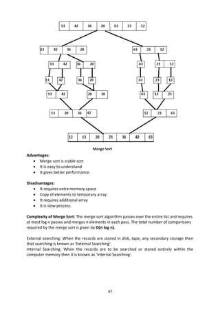
Example: Consider the following array with 6 elements. Sort the elements of the array by
using selection sort.
A = {10, 2, 3, 90, 43, 56}.
Sorted A = {2, 3, 10, 43, 56, 90}
Complexity
Complexity Best
Case
Average Case Worst Case
Time Ω(n) θ(n2
) o(n2
)
Space o(1)
Pass Pos A[0] A[1] A[2] A[3] A[4] A[5]
1 1 2 10 3 90 43 56
2 2 2 3 10 90 43 56
3 3 2 3 10 90 43 56
4 4 2 3 10 43 90 56
5 5 2 3 10 43 56 90

39
Algorithm
SELECTION SORT (ARR, N)
Step 1: Repeat Steps 2 and 3 for K = 1 to N-1
Step 2: CALL SMALLEST(A, K, N, POS)
Step 3: SWAP A[K] with
A[POS] [END OF LOOP]
Step 4: EXIT
BUBBLE SORT
Bubble Sort: This sorting technique is also known as exchange sort, which arranges
values by iterating over the list several times and in each iteration the larger value gets
bubble up to the end of the list. This algorithm uses multiple passes and in each pass the
first and second data items are compared. if the first data item is bigger than the second,
then the two items are swapped. Next the items in second and third position are compared
and if the first one is larger than the second, then they are swapped, otherwise no change in
their order. This process continues for each successive pair of data items until all items are
sorted.
Bubble Sort Algorithm:
Step 1: Repeat Steps 2 and 3 for i=1 to 10
Step 2: Set j=1
Step 3: Repeat while j<=n
(A)
if a[i] < a[j] Then
interchange a[i] and a[j]
[End of if]
(B) Set j = j+1
[End of Inner Loop]
[End of Step 1 Outer Loop]
Step 4: Exit

40
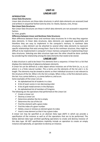
INSERTION SORT
Insertion sort is one of the best sorting techniques. It is twice as fast as Bubble sort.
In Insertion sort the elements comparisons are as less as compared to bubble sort. In this
comparison the value until all prior elements are less than the compared values is not
found. This means that all the previous values are lesser than compared value. Insertion
sort is good choice for small values and for nearly sorted values.
Working of Insertion sort:
The Insertion sort algorithm selects each element and inserts it at its proper position in a
sub list sorted earlier. In a first pass the elements A1 is compared with A0 and if A[1] and A[0]
are not sorted they are swapped.
In the second pass the element[2] is compared with A[0] and A[1]. And it is inserted at its
proper position in the sorted sub list containing the elements A[0] and A[1]. Similarly doing
ith
iteration the element A[i] is placed at its proper position in the sorted sub list, containing
the elements A[0],A[1],A[2],…………A[i-1].
To understand the insertion sort consider the unsorted Array A={7,33,20,11,6}.
The steps to sort the values stored in the array in ascending order using Insertion sort are
given below:

41
7 33 20 11 6
Step 1: The first value i.e; 7 is trivially sorted by itself.
Step 2: the second value 33 is compared with the first value 7. Since 33 is greater than 7, so
no changes are made.
Step 3: Next the third element 20 is compared with its previous element (towards left).Here
20 is less than 33.but 20 is greater than 7. So it is inserted at second position. For this 33 is
shifted towards right and 20 is placed at its appropriate position.
7 33 20 11 6
7 20 33 11 6
Step 4: Then the fourth element 11 is compared with its previous elements. Since 11 is less
than 33 and 20 ; and greater than 7. So it is placed in between 7 and 20. For this the
elements 20 and 33 are shifted one position towards the right.
7 20 33 11 6
7 11 20 33 6
Step5: Finally the last element 6 is compared with all the elements preceding it. Since it is
smaller than all other elements, so they are shifted one position towards right and 6 is
inserted at the first position in the array. After this pass, the Array is sorted.
7 11 20 33 6
6 7 11 20 33
Step 6: Finally the sorted Array is as follows:
6 7 11 20 33
ALGORITHM:
Insertion_sort(ARR,SIZE)
Step 1: Set i=1;
Step 2: while(i<SIZE)
Set temp=ARR[i]
J=i=1;
While(Temp<=ARR[j] and j>=0)
Set ARR[j+1]=ARR[i]
Set j=j-1
End While
SET ARR(j+1)=Temp;

42
Print ARR after ith
pass
Set i=i+1
End while
Step 3: print no.of passes i-1
Step 4: end
Advantages of Insertion Sort:
 It is simple sorting algorithm, in which the elements are sorted by considering one
item at a time. The implementation is simple.
 It is efficient for smaller data set and for data set that has been substantially sorted
before.
 It does not change the relative order of elements with equal keys
 It reduces unnecessary travels through the array
 It requires constant amount of extra memory space.
Disadvantages:-
 It is less efficient on list containing more number of elements.
 As the number of elements increases the performance of program would be slow
Complexity of Insertion Sort:
BEST CASE:-
Only one comparison is made in each pass.
The Time complexity is O(n2
).
WORST CASE:- In the worst case i.e; if the list is arranged in descending order, the number
of comparisons required by the insertion sort is given by:
1+2+3+……………………….+(n-2)+(n-1)= (n*(n-1))/2;
= (n2
-n)/2.
The number of Comparisons are O(n2
).
AVERAGE CASE:- In average case the numer of comparisons is given by
1
2
+
2
2
+
3
3
+ ⋯ +
(n−2)
2
+
(n−1)
2
=
n∗(n−1)
2∗2
=(n2
-n)/4 = O(n2
).
Program:
/* Program to implement insertion sort*/
#include<iostream.h>
#include<conio.h>
main()
{
int a[10],i,j,n,t;
clrscr();
cout<<”n Enter number of elements to be Sort:”;
cin>>n;
cout<<”n Enter the elements to be Sorted:”;
for(i=0;i<n;i++)
cin>>a[i];
for(i=0;i<n;i++)
{ t=a[i];
J=I;
while((j>0)&&(a[j-1]>t))
{ a[j]=a[j-1];

43
J=j-1;
}
a[j]=t;
}
cout<<”Array after Insertion sort:”;
for(i=0;i<n;i++)
cout<”n a[i]”;
getch();
}
OUTPUT:
Enter number of elements to sot:5
Enter number of elements to sorted: 7 33 20 11 6
Array after Insertion sort: 6 7 11 20 33.
QUICK SORT
The Quick Sort algorithm follows the principal of divide and Conquer. It first picks
up the partition element called ‘Pivot’, which divides the list into two sub lists such that all
the elements in the left sub list are smaller than pivot and all the elements in the right sub
list are greater than the pivot. The same process is applied on the left and right sub lists
separately. This process is repeated recursively until each sub list containing more than one
element.
Working of Quick Sort:
The main task in Quick Sort is to find the pivot that partitions the given list into two halves,
so that the pivot is placed at its appropriate position in the array. The choice of pivot as a
significant effect on the efficiency of Quick Sort algorithm. The simplest way is to choose the
first element as the Pivot. However the first element is not good choice, especially if the
given list is ordered or nearly ordered .For better efficiency the middle element can be
chosen as Pivot.
Initially three elements Pivot, Beg and End are taken, such that both Pivot and Beg refers to
0th
position and End refers to the (n-1)th
position in the list. The first pass terminates when
Pivot, Beg and End all refers to the same array element. This indicates that the Pivot
element is placed at its final position. The elements to the left of Pivot are smaller than this
element and the elements to it right are greater.
To understand the Quick Sort algorithm, consider an unsorted array as follows. The steps to
sort the values stored in the array in the ascending order using Quick Sort are given below.
8 33 6 21 4
Step 1: Initially the index ‘0’ in the list is chosen as Pivot and the index variable Beg and End
are initiated with index ‘0’ and (n-1) respectively.

44
Step 2: The scanning of the element starts from the end of the list.
A[Pivot]>A[End]
i.e; 8>4
so they are swapped.
Step 3: Now the scanning of the elements starts from the beginning of the list. Since
A[Pivot]>A[Beg]. So Beg is incremented by one and the list remains unchanged.
Step 4: The element A[Pivot] is smaller than A[Beg].So they are swapped.
Step 5: Again the list is scanned form right to left. Since A[Pivot] is smaller than A[End], so
the value of End is decreased by one and the list remains unchanged.
Step 6: Next the element A[Pivot] is smaller than A[End], the value of End is increased by
one. and the list remains unchanged.

45
Step 7: A[Pivot>>A[End] so they are swapped.
Step 8: Now the list is scanned from left to right. Since A[Pivot]>A[Beg],value of Beg is
increased by one and the list remains unchanged.
At this point the variable Pivot, Beg, End all refers to same element, the first pass is
terminated and the value 8 is placed at its appropriate position. The elements to its left are
smaller than 8 and the elements to its right are greater than 8.The same process is applied
on left and right sub lists.
ALGORITHM
Step 1: Select first element of array as Pivot
Step 2: Initialize i and j to Beg and End elements respectively
Step 3: Increment i until A[i]>Pivot.
Stop
Step 4: Decrement j until A[ j]>Pivot
Stop
Step 5: if i<j interchange A[i] with A[j].
Step 6: Repeat steps 3,4,5 until i>j i.e: i crossed j.
Step 7: Exchange the Pivot element with element placed at j, which is correct place for
Pivot.
Advantages of Quick Sort:
 This is fastest sorting technique among all.
 It efficiency is also relatively good.
 It requires small amount of memory
Disadvantages:
 It is somewhat complex method for sorting.
 It is little hard to implement than other sorting methods
 It does not perform well in the case of small group of elements.
Complexities of Quick Sort:
Average Case: The running time complexity is O(n log n).
Worst Case : Input array is not evenly divided. So the running time complexity is O(n2
).
Best Case: Input array is evenly divided. So the running time complexity is O(n logn).

46
MERGE SORT
The Merge Sort algorithm is based on the fact that it is easier and faster to sort two
smaller arrays than one large array. It follows the principle of “Divide and Conquered”. In
this sorting the list is first divided into two halves. The left and right sub lists obtained are
recursively divided into two sub lists until each sub list contains not more than one element.
The sub list containing only one element do not require any sorting. After that merge the
two sorted sub lists to form a combined list and recursively applies the merging process till
the sorted array is achieved.
Let us apply the Merge Sort to sort the following list:
13 42 36 20 63 23 12
Step 1: First divide the combined list into two sub lists as follows.
Step 2: Now Divide the left sub list into smaller sub list
Step 3: Similarly divide the sub lists till one element is left in the sub list.
Step 4: Next sort the elements in their appropriate positions and then combined the sub
lists.
Step 5: Now these two sub lists are again merged to give the following sorted sub list of size
4.
Step 6: After sorting the left half of the array, containing the same process for the right sub
list also. Then the sorted array of right half of the list is as follows.
Step 7: Finally the left and right halves of the array are merged to give the sorted array as
follows.

47
Advantages:
 Merge sort is stable sort
 It is easy to understand
 It gives better performance.
Disadvantages:
 It requires extra memory space
 Copy of elements to temporary array
 It requires additional array
 It is slow process.
Complexity of Merge Sort: The merge sort algorithm passes over the entire list and requires
at most log n passes and merges n elements in each pass. The total number of comparisons
required by the merge sort is given by O(n log n).
External searching: When the records are stored in disk, tape, any secondary storage then
that searching is known as ‘External Searching’.
Internal Searching: When the records are to be searched or stored entirely within the
computer memory then it is known as ‘Internal Searching’.

48
LINEAR SEARCH
The Linear search or Sequential Search is most simple searching method. It does
not expect the list to be sorted. The Key which to be searched is compared with each
element of the list one by one. If a match exists, the search is terminated. If the end of the
list is reached, it means that the search has failed and the Key has no matching element in
the list.
Ex: consider the following Array A
23 15 18 17 42 96 103
Now let us search for 17 by Linear search. The searching starts from the first position.
Since A[0] ≠17.
The search proceeds to the next position i.e; second position A[1] ≠17.
The above process continuous until the search element is found such as A[3]=17.
Here the searching element is found in the position 4.
Algorithm: LINEAR(DATA, N,ITEM, LOC)
Here DATA is a linear Array with N elements. And ITEM is a given item of information. This
algorithm finds the location LOC of an ITEM in DATA. LOC=-1 if the search is unsuccessful.
Step 1: Set DATA[N+1]=ITEM
Step 2: Set LOC=1
Step 3: Repeat while (DATA [LOC] != ITEM)
Set LOC=LOC+1
Step 4: if LOC=N+1 then
Set LOC= -1.
Step 5: Exit
Advantages:
 It is simplest known technique.
 The elements in the list can be in any order.
Disadvantages:
This method is in efficient when large numbers of elements are present in list because time
taken for searching is more.
Complexity of Linear Search: The worst and average case complexity of Linear search is
O(n), where ‘n’ is the total number of elements present in the list.
BINARY SEARCH
Suppose DATA is an array which is stored in increasing order then there is an extremely
efficient searching algorithm called “Binary Search”. Binary Search can be used to find the
location of the given ITEM of information in DATA.
Working of Binary Search Algorithm:
During each stage of algorithm search for ITEM is reduced to a segment of elements of
DATA[BEG], DATA[BEG+1], DATA[BEG+2],……………………… DATA[END].
Here BEG and END denotes beginning and ending locations of the segment under
considerations. The algorithm compares ITEM with middle element DATA[MID] of a
segment, where MID=[BEG+END]/2. If DATA[MID]=ITEM then the search is successful. and
we said that LOC=MID. Otherwise a new segment of data is obtained as follows:
i. If ITEM<DATA[MID] then item can appear only in the left half of the segment.
DATA[BEG], DATA[BEG+1], DATA[BEG+2]
So we reset END=MID-1. And begin the search again.

49
ii. If ITEM>DATA[MID] then ITEM can appear only in right half of the segment i.e.
DATA[MID+1], DATA[MID+2],……………………DATA[END].
So we reset BEG=MID+1. And begin the search again.
Initially we begin with the entire array DATA i.e. we begin with BEG=1 and END=n
Or
BEG=lb(Lower Bound)
END=ub(Upper Bound)
If ITEM is not in DATA then eventually we obtained END<BEG. This condition signals that the
searching is Unsuccessful.
The precondition for using Binary Search is that the list must be sorted one.
Ex: consider a list of sorted elements stored in an Array A is
Let the key element which is to be searched is 35.
Key=35
The number of elements in the list n=9.
Step 1: MID= [lb+ub]/2
=(1+9)/2
=5
Key<A[MID]
i.e. 35<46.
So search continues at lower half of the array.
Ub=MID-1
=5-1
= 4.
=(1+4)/2
=2.
Key>A[MID]
i.e. 35>12.
So search continues at Upper Half of the array.
Lb=MID+1
=2+1
= 3.

50
=(3+4)/2
=3.
Key>A[MID]
i.e. 35>30.
So search continues at Upper Half of the array.
Lb=MID+1
=3+1
= 4.
=(4+4)/2
=4.
ALGORITHM:
BINARY SEARCH[A,N,KEY]
Step 1: begin
Step 2: [Initilization]
Lb=1; ub=n;
Step 3: [Search for the ITEM]
Repeat through step 4,while Lower bound is less than Upper Bound.
Step 4: [Obtain the index of middle value]
MID=(lb+ub)/2
Step 5: [Compare to search for ITEM]
If Key<A[MID] then
Ub=MID-1
Other wise if Key >A[MID] then
Lb=MID+1
Otherwise write “Match Found”
Return Middle.
Step 6: [Unsuccessful Search]
write “Match Not Found”
Step 7: Stop.
Advantages: When the number of elements in the list is large, Binary Search executed faster
than linear search. Hence this method is efficient when number of elements is large.

51
Disadvantages: To implement Binary Search method the elements in the list must be in
sorted order, otherwise it fails.
Define sorting? What is the difference between internal and external sorting methods?
Ans:- Sorting is a technique of organizing data. It is a process of arranging the elements
either may be ascending or descending order, ie; bringing some order lines with data.
Internal sorting External sorting
1. Internal Sorting takes place in the main
memory of a computer.
1. External sorting is done with additional
external memory like magnetic tape or hard
disk
2. The internal sorting methods are applied
to small collection of data.
2. The External sorting methods are applied
only when the number of data elements to
be sorted is too large.
3. Internal sorting takes small input 3. External sorting can take as much as large
input.
4. It means that, the entire collection of data
to be sorted in small enough that the sorting
can take place within main memory.
4. External sorting typically uses a sort-
merge strategy, and requires auxiliary
storage.
5. For sorting larger datasets, it may be
necessary to hold only a chunk of data in
memory at a time, since it wont all fit.
5. In the sorting phase, chunks of data small
enough to fit in main memory are read,
sorted, and written out to a temporary file.
6. Example of Internal Sorting algorithms are
:- Bubble Sort, Internal Sort, Quick Sort,
Heap Sort, Binary Sort, Radix Sort, Selection
sort.
6. Example of External sorting algorithms
are: - Merge Sort, Two-way merge sort.
7. Internal sorting does not make use of
extra resources.
7. External sorting make use of extra
resources.
Justify the fact that the efficiency of Quick sort is O(nlog n) under best case?
Ans:- Best Case:-
The best case in quick sort arises when the pivot element divides the lists into two exactly
equal sub lists. Accordingly
i) Reducing the initial list places '1' element and produces two equal sub lists.
ii) Reducing the two sub lists places '2' elements and produces four equal sub lists and son
on.
Observe that the reduction step in the k th
level finals the location of 2(k-1)
elements, hence there will be approximately log n levels of reduction. Further, each level
uses at most 'n' comparisons, So f(n) = O(n log n).Hence the efficiency of quick sort
algorithm is O(nlog n) under the best case.
Mathematical Proof:- Hence from the above, the recurrence relation for quick sort under
best case is given by
T(n)=2T(n/2) + kn
By using substitution method , we get
T(n)=2T(n/2)+Kn
=2{ 2T(n/4)+k.n/2}+kn
=4T(n/4) + 2kn

52
.
.
.
In general
T(n)= 2k
T(n/2k
) + akn // after k substitutions
The above recurrence relation continues until n=2k
, k=logn
By substituting the above values , we get
T(n) is O(nlogn)
Quick sort, or partition-exchange sort, is a sorting algorithm that, on
average, makes O(n log n) comparisons to sort n items. In the worst case, it makes O(n2
)
comparisons, though this behavior is rare. Quick sort is often faster in practice than other
O(n log n) algorithms. Additionally, quick sort’s sequential and localized memory references
work well with a cache. Quick sort is a comparison sort and, in efficient implementations, is
not a stable sort. Quick sort can be implemented with an in-place partitioning algorithm, so
the entire sort can be done with only O(log n) additional space used by the stack during the
recursion. Since each element ultimately ends up in the correct position, the algorithm
correctly sorts. But how long does it take.
The best case for divide-and-conquer algorithms comes when we split the
input as evenly as possible. Thus in the best case, each sub problem is of size n/2.The
partition step on each sub problem is linear in its size. Thus the total effort in partitioning
the 2k
problems of size n/2k
is O(n).
The recursion tree for the best case looks like this:
The total partitioning on each level is O(n), and it take log n levels of perfect partitions to
get to single element sub problems. When we are down to single elements, the problems
are sorted. Thus the total time in the best case is O(nlogn) .

53
UNIT-V
TREES AND BINARY TREES
TREES
INTRODUCTION
In linear data structure data is organized in sequential order and in non-linear data structure
data is organized in random order. A tree is a very popular non-linear data structure used in
a wide range of applications. Tree is a non-linear data structure which organizes data in
hierarchical structure and this is a recursive definition.
DEFINITION OF TREE:
Tree is collection of nodes (or) vertices and their edges (or) links. In tree data structure,
every individual element is called as Node. Node in a tree data structure stores the actual
data of that particular element and link to next element in hierarchical structure.
Note: 1. In a Tree, if we have N number of nodes then we can have a maximum of N-
1 number of links or edges.
2. Tree has no cycles.
TREE TERMINOLOGIES:
1. Root Node: In a Tree data structure, the first node is called as Root Node. Every tree
must have a root node. We can say that the root node is the origin of the tree data
structure. In any tree, there must be only one root node. We never have multiple root
nodes in a tree.
2. Edge: In a Tree, the connecting link between any two nodes is called as EDGE. In a tree
with 'N' number of nodes there will be a maximum of 'N-1' number of edges.

54
3. Parent Node: In a Tree, the node which is a predecessor of any node is called as PARENT
NODE. In simple words, the node which has a branch from it to any other node is called a
parent node. Parent node can also be defined as "The node which has child / children".
Here, A is parent of B&C. B is the parent of D,E&F and so on…
4. Child Node: In a Tree data structure, the node which is descendant of any node is called
as CHILD Node. In simple words, the node which has a link from its parent node is called as
child node. In a tree, any parent node can have any number of child nodes. In a tree, all the
nodes except root are child nodes.
5. Siblings: In a Tree data structure, nodes which belong to same Parent are called
as SIBLINGS. In simple words, the nodes with the same parent are called Sibling nodes.

55
6. Leaf Node: In a Tree data structure, the node which does not have a child is called
as LEAF Node. In simple words, a leaf is a node with no child. In a tree data structure, the
leaf nodes are also called as External Nodes. External node is also a node with no child. In a
tree, leaf node is also called as 'Terminal' node.
7. Internal Nodes: In a Tree data structure, the node which has atleast one child is called
as INTERNAL Node. In simple words, an internal node is a node with atleast one child.
In a Tree data structure, nodes other than leaf nodes are called as Internal Nodes. The root
node is also said to be Internal Node if the tree has more than one node. Internal nodes are
also called as 'Non-Terminal' nodes.
8. Degree: In a Tree data structure, the total number of children of a node is called
as DEGREE of that Node. In simple words, the Degree of a node is total number of children it
has. The highest degree of a node among all the nodes in a tree is called as 'Degree of Tree'
Degree of Tree is: 3
9. Level: In a Tree data structure, the root node is said to be at Level 0 and the children of
root node are at Level 1 and the children of the nodes which are at Level 1 will be at Level 2

56
and so on... In simple words, in a tree each step from top to bottom is called as a Level and
the Level count starts with '0' and incremented by one at each level (Step).
10. Height: In a Tree data structure, the total number of edges from leaf node to a particular
node in the longest path is called as HEIGHT of that Node. In a tree, height of the root node
is said to be height of the tree. In a tree, height of all leaf nodes is '0'.
11. Depth: In a Tree data structure, the total number of egdes from root node to a
particular node is called as DEPTH of that Node. In a tree, the total number of edges from
root node to a leaf node in the longest path is said to be Depth of the tree. In simple words,
the highest depth of any leaf node in a tree is said to be depth of that tree. In a tree, depth
of the root node is '0'.
12. Path: In a Tree data structure, the sequence of Nodes and Edges from one node to
another node is called as PATH between that two Nodes. Length of a Path is total number
of nodes in that path. In below example the path A - B - E - J has length 4.

57
13. Sub Tree: In a Tree data structure, each child from a node forms a subtree recursively.
Every child node will form a subtree on its parent node.
TREE REPRESENTATIONS:
A tree data structure can be represented in two methods. Those methods are as follows...
1. List Representation
2. Left Child - Right Sibling Representation
Consider the following tree...
1. List Representation
In this representation, we use two types of nodes one for representing the node with data
called 'data node' and another for representing only references called 'reference node'. We
start with a 'data node' from the root node in the tree. Then it is linked to an internal node

58
through a 'reference node' which is further linked to any other node directly. This process
repeats for all the nodes in the tree.
The above example tree can be represented using List representation as follows...
2. Left Child - Right Sibling Representation
In this representation, we use a list with one type of node which consists of three fields
namely Data field, Left child reference field and Right sibling reference field. Data field
stores the actual value of a node, left reference field stores the address of the left child and
right reference field stores the address of the right sibling node. Graphical representation of
that node is as follows...
In this representation, every node's data field stores the actual value of that node. If that node has
left a child, then left reference field stores the address of that left child node otherwise stores NULL.
If that node has the right sibling, then right reference field stores the address of right sibling node
otherwise stores NULL.
The above example tree can be represented using Left Child - Right Sibling representation as
follows...
BINARY TREE:
In a normal tree, every node can have any number of children. A binary tree is a special type
of tree data structure in which every node can have a maximum of 2 children. One is known
as a left child and the other is known as right child.
A tree in which every node can have a maximum of two children is called Binary Tree.

59
In a binary tree, every node can have either 0 children or 1 child or 2 children but not more
than 2 children.
In general, tree nodes can have any number of children. In a binary tree, each node can
have at most two children. A binary tree is either empty or consists of a node called the root
together with two binary trees called the left subtree and the right subtree. A tree with no
nodes is called as a null tree
Example:
TYPES OF BINARY TREE:
1. Strictly Binary Tree:
In a binary tree, every node can have a maximum of two children. But in strictly binary tree,
every node should have exactly two children or none. That means every internal node must
have exactly two children. A strictly Binary Tree can be defined as follows...
A binary tree in which every node has either two or zero number of children is called
Strictly Binary Tree
Strictly binary tree is also called as Full Binary Tree or Proper Binary Tree or 2-Tree.
Strictly binary tree data structure is used to represent mathematical expressions.

60
Example
2. Complete Binary Tree:
In a binary tree, every node can have a maximum of two children. But in strictly binary tree,
every node should have exactly two children or none and in complete binary tree all the
nodes must have exactly two children and at every level of complete binary tree there must
be 2level
number of nodes. For example at level 2 there must be 22
= 4 nodes and at level 3
there must be 23
= 8 nodes.
A binary tree in which every internal node has exactly two children and all leaf nodes are
at same level is called Complete Binary Tree.
Complete binary tree is also called as Perfect Binary Tree.
3. Extended Binary Tree:
A binary tree can be converted into Full Binary tree by adding dummy nodes to existing
nodes wherever required.
The full binary tree obtained by adding dummy nodes to a binary tree is called as
Extended Binary Tree.

61
In above figure, a normal binary tree is converted into full binary tree by adding dummy
nodes.
4. Skewed Binary Tree:
If a tree which is dominated by left child node or right child node, is said to be a Skewed
Binary Tree.
In a skewed binary tree, all nodes except one have only one child node. The remaining
node has no child.
In a left skewed tree, most of the nodes have the left child without corresponding right
child.
In a right skewed tree, most of the nodes have the right child without corresponding left
child.
Properties of binary trees:
Some of the important properties of a binary tree are as follows:
1. If h = height of a binary tree, then
a. Maximum number of leaves = 2h
b. Maximum number of nodes = 2h + 1 - 1
2. If a binary tree contains m nodes at level l, it contains at most 2m nodes at level l + 1.
3. Since a binary tree can contain at most one node at level 0 (the root), it can contain at
most 2l node at level l.
4. The total number of edges in a full binary tree with n node is n –
BINARY TREE REPRESENTATIONS:
A binary tree data structure is represented using two methods. Those methods are as
follows...
1. Array Representation
2. Linked List Representation
Consider the following binary tree...

62
1. Array Representation of Binary Tree
In array representation of a binary tree, we use one-dimensional array (1-D Array) to
represent a binary tree.
Consider the above example of a binary tree and it is represented as follows...
To represent a binary tree of depth 'n' using array representation, we need one dimensional
array with a maximum size of 2n + 1
.
2. Linked List Representation of Binary Tree
We use a double linked list to represent a binary tree. In a double linked list, every node
consists of three fields. First field for storing left child address, second for storing actual
data and third for the right child address.
In this linked list representation, a node has the following structure...
The above example of the binary tree represented using Linked list representation is shown
as follows...
BINARY TREE TRAVERSALS:
Unlike linear data structures (Array, Linked List, Queues, Stacks, etc) which have only one
logical way to traverse them, binary trees can be traversed in different ways. Following are
the generally used ways for traversing binary trees.
When we wanted to display a binary tree, we need to follow some order in which all the
nodes of that binary tree must be displayed. In any binary tree, displaying order of nodes
depends on the traversal method.
Displaying (or) visiting order of nodes in a binary tree is called as Binary Tree Traversal.
There are three types of binary tree traversals.
1. In - Order Traversal
2. Pre - Order Traversal
3. Post - Order Traversal
1. In - Order Traversal (left Child - root - right Child):

63
In In-Order traversal, the root node is visited between the left child and right child. In this
traversal, the left child node is visited first, then the root node is visited and later we go for
visiting the right child node. This in-order traversal is applicable for every root node of all
sub trees in the tree. This is performed recursively for all nodes in the tree.
Algorithm:
Step-1: Visit the left subtree, using inorder.
Step-2: Visit the root.
Step-3: Visit the right subtree, using inorder.
In the above example of a binary tree, first we try to visit left child of root node 'A', but A's
left child 'B' is a root node for left subtree. so we try to visit its (B's) left child 'D' and again D
is a root for subtree with nodes D, I and J. So we try to visit its left child 'I' and it is the
leftmost child. So first we visit 'I' then go for its root node 'D' and later we visit D's right
child 'J'. With this we have completed the left part of node B. Then visit 'B' and next B's right
child 'F' is visited. With this we have completed left part of node A. Then visit root node 'A'.
With this we have completed left and root parts of node A. Then we go for the right part of
the node A. In right of A again there is a subtree with root C. So go for left child of C and
again it is a subtree with root G. But G does not have left part so we visit 'G' and then visit
G's right child K. With this we have completed the left part of node C. Then visit root
node 'C' and next visit C's right child 'H' which is the rightmost child in the tree. So we stop
the process.
That means here we have visited in the order of I - D - J - B - F - A - G - K - C - H using In-
Order Traversal.
2. Pre - Order Traversal ( root - leftChild - rightChild ):
In Pre-Order traversal, the root node is visited before the left child and right child nodes. In
this traversal, the root node is visited first, then its left child and later its right child. This pre-
order traversal is applicable for every root node of all subtrees in the tree. Preorder search
is also called backtracking.
Algorithm:
Step-2: Visit the left subtree, using preorder.
Step-3: Visit the right subtree, using preorder.

64
In the above example of binary tree, first we visit root node 'A' then visit its left
child 'B' which is a root for D and F. So we visit B's left child 'D' and again D is a root for I and
J. So we visit D's left child 'I' which is the leftmost child. So next we go for visiting D's right
child 'J'. With this we have completed root, left and right parts of node D and root, left parts
of node B. Next visit B's right child 'F'. With this we have completed root and left parts of
node A. So we go for A's right child 'C' which is a root node for G and H. After visiting C, we
go for its left child 'G' which is a root for node K. So next we visit left of G, but it does not
have left child so we go for G's right child 'K'. With this, we have completed node C's root
and left parts. Next visit C's right child 'H' which is the rightmost child in the tree. So we stop
the process.
That means here we have visited in the order of A-B-D-I-J-F-C-G-K-H using Pre-Order
Traversal.
3. Post - Order Traversal ( leftChild - rightChild - root ):
In Post-Order traversal, the root node is visited after left child and right child. In this
traversal, left child node is visited first, then its right child and then its root node. This is
recursively performed until the right most nodes are visited.
Algorithm:
Step-1: Visit the left subtree, using postorder.
Step-2: Visit the right subtree, using postorder
Here we have visited in the order of I - J - D - F - B - K - G - H - C - A using Post-Order
Traversal.

66
PROGRAMS ON DATA STRUCTURES
1. Write a C program to implement stack using arrays.
2. Write a C program to implement queue using arrays.
3. Write a C program implement the following Stack applications
a) infix into postfix
b) Evaluation of the postfix expression
4. Write a C program to implement the following types of queues
a) Priority queue
b) Circular queue
5. Write a C program to implement the Singly Linked List
6. Write a C program to implement the doubly Linked List
7. Write a C program to implement the following search algorithms.
i) Linear search ii) Binary search iii) Fibonacci search
8. Write a C program to implement the sorting algorithms.
9. Write a C program to implement binary tree using arrays and to perform binary
traversals.
i) Inorder ii) preorder iii) post order
10. Write a C program to balance a given tree.

67
1: STACK USING ARRAYS
#include<stdio.h>
#include<conio.h>
#include<process.h>
int ch,max,item,top=-1,s[20]; void menu(void);
void push(int); int pop(void); void display(void); void main()
{
clrscr();
printf("ENTER STACK SIZE:"); scanf("%d",&max);
menu();
getch();
}
void menu()
{
printf("1.PUSHn2.POPn3.EXITn"); printf("ENTER YOUR CHOICE:");
fflush(stdin);
scanf("%d",&ch);
switch(ch)
{
case 1:printf("ENTER THE ELEMENTn"); scanf("%d",&item);
push(item);
menu();
break;
case 2:item=pop(); menu();
break;
case 3:exit(0);
}
}
void push(int item)
{
if(top==max-1)
printf("STACK IS OVER FLOWn"); else
{
top++;
s[top]=item;
}
display();
}
int pop()
{
if(top==-1)
{
printf("STACK IS UNDER FLOWn"); return 0;
}
else
{
item=s[top]; top--;
}
display(); return item;

68
}
void display()
{
int i;
printf(" top -->");
for(i=top;i>=0;i--)
printf("%dnt",s[i]);
}
OUTPUT:
Enter stack size: 3
1. Push
2. Pop
3. Exit
Enter your choice:1
Enter the element: 3
Top: 3
1. Push
2. Pop
3. Exit
Enter your choice:1
Top: 5
3
1. Push
2. Pop
3. Exit
Enter your choice:1
Top: 9 5 3
1. Push
2. Pop
3. Exit
Enter your choice: 1
Stack is overflow
Top: 9 5 3
1. Push
2. Pop
3. Exit
Popped element is: 9
Top: 5 3
1. Push
2. Pop
3. Exit
Popped element is: 5
Top: 3
1. Push

69
2. Pop
3. Exit
Enter your choice: 2 Stack is underflow
1. Push
2. Pop
3. Exit
2. QUEUE USING ARRAYS
#include<stdio.h>
#include<conio.h>
#include<stdlib.h> void insertion(void); void deletion(void); void display(void);
int q[10],n,i,f,r;
int f=0,r=0; void main()
{
int op;
clrscr();
printf("ENTER THE SIZE OF QUEUE:"); scanf("%d",&n);
while(1)
{
printf("n1.INSERTIONn2.DELETIONn3.DISPLAYn4.EXITn");
printf("ENTER YOUR OPTION:");
scanf("%d",&op);
switch(op)
{
case 1:insertion(); break;
case 2:deletion(); break;
case 3:display(); break; default:exit(0);
} } }
void insertion()
{
if(r>=n)
printf("QUEUE IS OVER FLOW"); else
{
r=r+1;
printf("nENTER AN ELEMENT TO INSERT:"); scanf("%d",&q[r]);
if(f==0)
f=1;
} }
void deletion()
{
if(f==0)
printf("THE QUEUE IS EMPTY"); else
{
printf("THE DELETING ELEMENT IS:%5d",q[f]); f=f+1;
if(f>r)
f=0,r=0;
} }

70
void display()
{
if(f==0)
printf("QUEUE IS EMPTY"); else
for(i=f;i<=r;i++)
printf("%5d",q[i]);
}
OUTPUT:
Enter the size of queue: 2
1. Insertion
2. Deletion
3. Display
4. Exit
Enter your option: 1
Enter an element to insert: q [1]:34
1. Insertion
2. Deletion
3. Display
4. Exit
Enter your option: 3 34
1. Insertion
2. Deletion
3. Display
4. Exit
Enter your option: 4
3: STACK APPLICATIONS
a) INFIX INTO POSTFIX
b) EVALUATION OF THE POSTFIX EXPRESSION
Program:(a)
#include<stdio.h>
#include<conio.h>
#define MAX 50
char stack[MAX];
int top=-1
void push(char); char pop();
int priority(char); void main()
{
char a[MAX],ch; int i;
clrscr();
printf("Enter an infix expression:t"); gets(a);
printf("the postfix expression for the given expression is:t"); for(i=0;a[i]!='0';i++)
{
ch=a[i];
if((ch>='a') && (ch<='z')) printf("%c",ch);
else if(ch=='(') push(ch); else if(ch==')')
{

71
while((ch=pop())!='(')
printf("%c",ch);
}
else
{
while(priority(stack[top])>priority(ch))
printf("%c",pop());
push(ch);
}
}
while(top>-1) printf("%c",pop());
printf("n");
getch();
}
void push(char ch)
{
if(top==MAX-1)
{
printf("STACK OVERFLOW"); return;
}
else
{
top++;
stack[top]=ch; } }
char pop()
{
int x; if(top==-1)
{
printf("STACK EMPTY");
}
else
{ x=stack[top]; top--; }
return x;
}
int priority(char ch)
{
switch(ch)
{
case '^': return 4; case '*':
case '/': return 3; case '+':
case '-': return 2; default : return 0;
} }
OUTPUT:
Enter an infix expression:
((a + b ((b ^ c – d))) * (e – (a / c)))
The postfix expression for the given expression is:
a b b c ^ d - + e a c / - *

72
Program:(b)
#include<stdio.h>
#include<conio.h>
#include<math.h>
#include<ctype.h>
void push(char);
char pop(void);
char ex[50],s[50],op1,op2; int i,top=-1;
void main()
{
clrscr();
printf("Enter the expression:"); gets(ex); for(i=0;ex[i]!='0';i++)
{
if(isdigit(ex[i])) push(ex[i]-48); else
{
op2=pop();
op1=pop();
switch(ex[i])
{
case '+':push(op1+op2);
break;
case '-':push(op1-op2);
break;
case '*':push(op1*op2);
break;
case '/':push(op1/op2);
break;
case '%':push(op1%op2);
break;
case '^':push(pow(op1,op2));
break;
} } }
printf("result is :%d",s[top]); getch();
}
void push(char a)
{ s[++top]=a; }
char pop()
{ return(s[top--]);
}
OUTPUT:
Enter the expression: 384 * 2 / +83----
Result is: 14

73
4: TYPES OF QUEUES
a).Priority queue
b).Circular queue
Program: (a)
#include<stdio.h>
#include<conio.h>
#include<malloc.h>
typedef struct node
{
int priority;
int info;
struct node *link;
}n;
n *getnode()
{
return ( (n *)malloc(sizeof(n)));
}
n*front=NULL,*temp=NULL,*ptr=NULL,*q=NULL;
void insertion();
void deletion();
void display();
void main()
{
int ch;
clrscr();
printf("tMenun1.Insertionn2.Deletionn3.Displayn4.exit");
while(1)
{
printf("Enter your choice");
scanf("%d",&ch);
switch(ch)
{
case 1:insertion();
break;
case 2:deletion();
break;
case 3:display();
break;
case 4:exit();
default : printf("nInvalid choice ");
break;
} } }
void insertion()
{ int item,item_prty;
temp=getnode();
printf("Enter item to insert ");
scanf("%d",&item);
printf("Enter item prority ");

74
scanf("%d",&item_prty);
temp->priority=item_prty;
temp->info=item;
if(front==NULL||item_prty>front->priority)
{
temp->link=front;
front=temp;
}
else
{
q=front;
while (q->link!=NULL &&q->link-> priority >=item_prty)
q=q->link;
temp->link=q->link;
q->link=temp;
}
}
void deletion()
{ if(front==NULL)
printf("Queue is underflow");
else
{
temp=front;
printf("Deleted item is %dn",
temp->info);
front=front->link;
free(temp);
}
}
void display()
{
ptr=front;
if(front==NULL)
printf("Queue is underflow");
else
{
printf("Queue is :n");
printf("priority item :n");
while(ptr!=NULL)
{
printf("%5d %5dn",ptr->priority,ptr->info);
ptr=ptr->link;
}
}
}
OUTPUT:

75
1 - Insert an element into queue
2 - Delete an element from queue
3 - Display queue elements
4 - Exit
Enter value to be inserted: 20
89 45 20
89 56 45 20
Enter value to delete: 45
89 56 20
Program: (b)
#include<stdio.h>
#include<conio.h>
#define max 3
int q[max],rear=-1,front=-1;
void main()
{ int ch;
clrscr();
do
{ printf("nqueue implementationn");
printf("1.insert 2.delete 3.display 4.exitn");
printf("enter your choicen");
scanf("%d",&ch);
switch(ch)
{ case 1:insert(); break;
case 2:delete(); break;
case 3:display(); break;
case 4:exit(1);
default:printf("wrong choicen"); break;
}
}while(ch<=4);
getch();
}
insert()
{ int item;

76
if(rear==max-1)
{ printf("queue overflown"); }
else
{ if(front==-1)
front=0;
printf("insert the element in queue:");
scanf("%d",&item);
rear++;
q[rear]=item;
}
}
delete()
{ if(front==-1)
{ printf("queue underflown");
}
else
{ printf("element deleted from queue is:%dn",q[front]);
front++;
if(front==max)
front=rear=-1;
}
}
display()
{ int i;
if(front==-1)
printf("queue is emptyn");
else
{ printf("queue is :n");
for(i=front;;i++)
{ printf("%2d",q[i]);
if(i==rear)
return;
} } }
OUTPUT:
1. Insert
2. Delete
3. Display
4. Exit
Enter your choice:1
Enter element to cqueue: 10
1. Insert
2. Delete
3. Display
4. Exit
Enter element to circular queue: 20
1. Insert
2. Delete

77
3. Display
4. Exit
Deleted element from circular queue is: 10
1. Insert
2. Delete
3. Display
4. Exit
Elements from circular queue is: 20
1. Insert
2. Delete
3. Display
4. Exit
5: SINGLY LINKED LIST
Program:
#include<stdio.h>
#include<conio.h>
#include<stdlib.h>
#include<alloc.h> struct node
{
int data;
struct node* link; };
typedef struct node* pnode; pnode head=NULL;
void menu(void); void insbeg(int); void delbeg(void); void insend(int); void delend(void);
void insafter(int,int); void delmid(int); void display(void); void main()
{
int ch,x,pos; clrscr(); while(1)
{
menu();
printf("enter ur choicen"); scanf("%d",&ch);
switch(ch)
{
case 1: printf("enter element to insertn");
scanf("%d",&x);
insbeg(x);
break;
case 2:delbeg();
break;
case 3: printf("enter element to insertn");
scanf("%d",&x);
insend(x);
break;
case 4:delend();
break;
case 5: printf("enter element,pos to insertn");

DATA STRUCTURE.pdf

Recommended

Recommended

More Related Content

What's hot

What's hot (20)

Similar to DATA STRUCTURE.pdf

Similar to DATA STRUCTURE.pdf (20)

Recently uploaded

Recently uploaded (20)

DATA STRUCTURE.pdf