Design & analysis of algorithm

1. Design & Analysis of Algorithms (DAA)
B.Tech (5th
Sem)
By: Ms. Simran Arora

2. Course Content
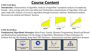
UNIT I (15 Hrs)
Introduction: Characteristics of algorithm. Analysis of algorithm: Asymptotic analysis of complexity
bounds – best, average and worst-case behaviour; Performance measurements of Algorithm, Time and
space trade-offs, Analysis of recursive algorithms through recurrence relations: Substitution method,
Recursion tree method and Masters’ theorem.
UNIT II (15 Hrs)
Fundamental Algorithmic Strategies: Brute-Force, Greedy, Dynamic Programming, Branch and Bound
and Backtracking methodologies for the design of algorithms; Illustrations of these techniques for
Problem Solving, Bin Packing, Knap Sack TSP. Heuristics –characteristics and their application domains.

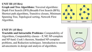
3. UNIT III (15 Hrs)
Graph and Tree Algorithms: Traversal algorithms:
Depth First Search (DFS),Breadth First Search (BFS);
Shortest path algorithms, Transitive closure, Minimum
Spanning Tree, Topological sorting, Network Flow
Algorithm.
UNIT IV (15 Hrs)
Tractable and Intractable Problems: Computability of
Algorithms, Computability classes – P, NP, NP-complete
and NP-hard. Cook’s theorem, Standard NP-complete
problems, and Reduction techniques. Introduction to recent
advancements in design and analysis of algorithms.

4. Recommended books:
• “Introduction to the design & Analysis of Algorithms” by Anany Levitin (Pearson education-
Third Edition)
• “Design & Analysis of Algorithms” by Biswajit R Bhowmik (S.K. Kataria & Sons- IInd
Edition(2012))
• “Introduction to Algorithms” by Thomas H. Cormen & Clifford Stein(MIT Press-1st
edition-
1990)
E-Books: duke.edu , freecomputerbooks.com
MOOC: NPTEL –Design and Analysis of Algorithms
https://nptel.ac.in/courses/106106131
Online Platform: geeksforgeeks , tutorialspoint

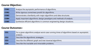
5. Course Objective:-
COB1 Analyze the asymptotic performance of algorithms.
COB2 Write rigorous correctness proofs for algorithms.
COB3 Demonstrate a familiarity with major algorithms and data structures.
COB4 Apply important algorithmic design paradigms and methods of analysis.
COB5 Synthesize efficient algorithms in common engineering design situations.
Course Outcomes:-
CO1 For a given algorithms analyze worst-case running times of algorithms based on asymptotic
analysis.
CO2 Describe the algorithmic strategies.
CO3 Describe the different graph and tree traversal algorithms.
CO4 Describe the tractable and intractable problems.

6. Structure:-

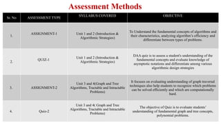
7. Assessment Methods
Sr. No ASSESSMENT TYPE
SYLLABUS COVERED OBJECTIVE
1.
ASSIGNMENT-1 Unit 1 and 2 (Introduction &
Algorithmic Strategies)
To Understand the fundamental concepts of algorithms and
their characteristics, analyzing algorithm’s efficiency and
differentiate between types of problems.
2.
QUIZ-1
Unit 1 and 2 (Introduction &
Algorithmic Strategies)
DAA quiz is to assess a student's understanding of the
fundamental concepts and evaluate knowledge of
asymptotic notations and differentiate among various
algorithmic design strategies
3. ASSIGNMENT-2
Unit 3 and 4(Graph and Tree
Algorithms, Tractable and Intractable
Problems)
It focuses on evaluating understanding of graph traversal
techniques also help students to recognize which problems
can be solved efficiently and which are computationally
hard.
4. Quiz-2
Unit 3 and 4( Graph and Tree
Algorithms, Tractable and Intractable
Problems)
The objective of Quiz is to evaluate students’
understanding of fundamental graph and tree concepts,
polynomial problems.

8. Sr.
No
Assessment type Covered topics Objective
5
MST- 1
Unit 1 and 2 (Introduction & Algorithmic
Strategies)
Mid-semester exam is to assess a student's understanding of
the fundamental concepts and design of algorithms using
different methodologies.
6
MST-2
Unit 3 and 4( Graph and Tree Algorithms,
Tractable and Intractable Problems)
Mid-semester exam is to assess a student's understanding of
the fundamental principles of advance design and analysis of
algorithm using different techniques.
7.
STUDENT
PRESENTATIONS Mini-projects and Assigned topic
To enhance conceptual understanding and communication
skills. It aims to develop critical thinking and collaborative
learning.
8. FINAL EXAMINATION
Whole syllabus
The objective of the final exam is to assess the overall
understanding, analytical ability, and application skills of
students acquired throughout the course.

9. Why do we study Design & Analysis of
Algorithm?
• Benefits of Algorithm
Logic is developed before actual coding.
• Benefits of Analysis of Algorithm
To find best version of solution from
various solution of same problem
• Benefits of Design of Algorithm
To create an efficient algorithm to solve
a problem in an efficient way.

10. Introduction
An Algorithm is a set of rules that must be followed when solving a specific problem. We can also define an
algorithm as a well defined computational procedure which takes some value or set of values as input and
generates output. The result of a given problem is the output for a given problem.
It acts like a set of instructions on how a program should be executed. Thus, there is no fixed structure of an
algorithm. The main aim of designing an algorithm is to provide a optimal solution for a problem. Not all
problems must have similar type of solutions; an optimal solution for one problem may not be optimal for
another. Therefore, we must adopt various strategies to provide feasible solutions for all types of problems.

11. Real Life Applications of Algorithm
Examples include following a recipe to bake a cake, using a GPS to find the fastest route, or even something as simple as tying your shoes.
1. Cooking Recipes: Recipes are a classic example of an algorithm. They provide a detailed list of steps and ingredients needed to prepare a
dish. The steps must be followed in order to produce the desired result.
2. Driving Directions: When using a GPS or map app, you're essentially following an algorithm that calculates the optimal route to your
destination, taking into account factors like traffic and road closures.
3. Online Shopping: The entire process of online shopping, from adding items to your cart to completing the purchase, involves a series of
algorithms that manage inventory, payments, and shipping.
4. Social Media Recommendations: Social media platforms use algorithms to suggest friends, content, and advertisements based on your
activity and preferences.
5. Search Engines: When you search for something online, search engines use algorithms to crawl the web, index pages, and rank them
based on relevance to your query.

12. Use of Algorithms
Computer Science: Algorithms form the basis of computer programming and are used to solve problems ranging
from simple sorting and searching to complex tasks such as artificial intelligence and machine learning.
Mathematics: Algorithms are used to solve mathematical problems, such as finding the optimal solution to a system
of linear equations or finding the shortest path in a graph.
Operations Research: Algorithms are used to optimize and make decisions in fields such as transportation, logistics,
and resource allocation.
Artificial Intelligence: Algorithms are the foundation of artificial intelligence and machine learning, and are used to
develop intelligent systems that can perform tasks such as image recognition, natural language processing, and
decision-making.
Data Science: Algorithms are used to analyze, process, and extract insights from large amounts of data in fields such
as marketing, finance, and healthcare.

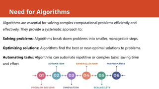
13. Need for Algorithms
Algorithms are essential for solving complex computational problems efficiently and
effectively. They provide a systematic approach to:
Solving problems: Algorithms break down problems into smaller, manageable steps.
Optimizing solutions: Algorithms find the best or near-optimal solutions to problems.
Automating tasks: Algorithms can automate repetitive or complex tasks, saving time
and effort.

14. Characteristics for Algorithm

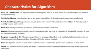
15. Clear and Unambiguous: The algorithm should be unambiguous. Each of its steps should be clear in all aspects and must lead
to only one meaning.
Well-Defined Inputs: If an algorithm says to take inputs, it should be well-defined inputs. It may or may not take input.
Well-Defined Outputs: The algorithm must clearly define what output will be yielded and it should be well-defined as well. It
should produce at least 1 output.
Finite-ness: The algorithm must be finite, i.e. it should terminate after a finite time.
Feasible: The algorithm must be simple, generic, and practical, such that it can be executed with the available resources. It must
not contain some future technology
Language Independent: The Algorithm designed must be language-independent, i.e. it must be just plain instructions that can
be implemented in any language, and yet the output will be the same, as expected.
Input: An algorithm has zero or more inputs. Each that contains a fundamental operator must accept zero or more inputs.
Output: An algorithm produces at least one output. Every instruction that contains a fundamental operator must accept zero or
more inputs.
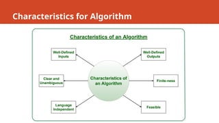
Characteristics for Algorithm

16. Designing of an Algorithm

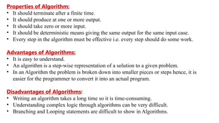
17. Properties of Algorithm:
• It should terminate after a finite time.
• It should produce at one or more output.
• It should take zero or more input.
• It should be deterministic means giving the same output for the same input case.
• Every step in the algorithm must be effective i.e. every step should do some work.
Advantages of Algorithms:
• It is easy to understand.
• An algorithm is a step-wise representation of a solution to a given problem.
• In an Algorithm the problem is broken down into smaller pieces or steps hence, it is
easier for the programmer to convert it into an actual program.
Disadvantages of Algorithms:
• Writing an algorithm takes a long time so it is time-consuming.
• Understanding complex logic through algorithms can be very difficult.
• Branching and Looping statements are difficult to show in Algorithms.

18. Algorithm Design Analysis of Algorithm
Two Main task in the study of algorithms

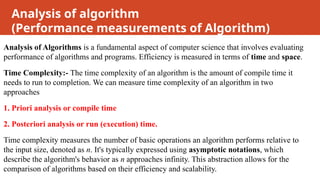
19. Analysis of algorithm
(Performance measurements of Algorithm)
Analysis of Algorithms is a fundamental aspect of computer science that involves evaluating
performance of algorithms and programs. Efficiency is measured in terms of time and space.
Time Complexity:- The time complexity of an algorithm is the amount of compile time it
needs to run to completion. We can measure time complexity of an algorithm in two
approaches
1. Priori analysis or compile time
2. Posteriori analysis or run (execution) time.
Time complexity measures the number of basic operations an algorithm performs relative to
the input size, denoted as n. It's typically expressed using asymptotic notations, which
describe the algorithm's behavior as n approaches infinity. This abstraction allows for the
comparison of algorithms based on their efficiency and scalability.

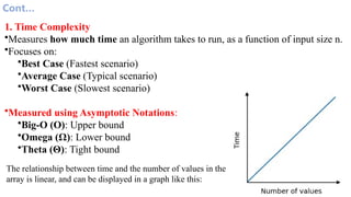
20. Cont…
The relationship between time and the number of values in the
array is linear, and can be displayed in a graph like this:
1. Time Complexity
•Measures how much time an algorithm takes to run, as a function of input size n.
•Focuses on:
•Best Case (Fastest scenario)
•Average Case (Typical scenario)
•Worst Case (Slowest scenario)
•Measured using Asymptotic Notations:
•Big-O (O): Upper bound
•Omega (Ω): Lower bound
•Theta (Θ): Tight bound

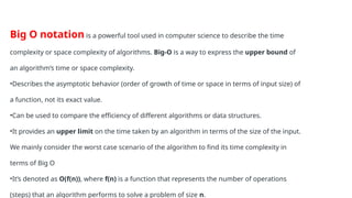
21. Big O notation is a powerful tool used in computer science to describe the time
complexity or space complexity of algorithms. Big-O is a way to express the upper bound of
an algorithm’s time or space complexity.
•Describes the asymptotic behavior (order of growth of time or space in terms of input size) of
a function, not its exact value.
•Can be used to compare the efficiency of different algorithms or data structures.
•It provides an upper limit on the time taken by an algorithm in terms of the size of the input.
We mainly consider the worst case scenario of the algorithm to find its time complexity in
terms of Big O
•It’s denoted as O(f(n)), where f(n) is a function that represents the number of operations
(steps) that an algorithm performs to solve a problem of size n.

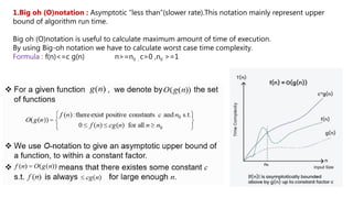
22. 1.Big oh (O)notation : Asymptotic “less than”(slower rate).This notation mainly represent upper
bound of algorithm run time.
Big oh (O)notation is useful to calculate maximum amount of time of execution.
By using Big-oh notation we have to calculate worst case time complexity.
Formula : f(n)<=c g(n) n>=n0 , c>0 ,n0 >=1

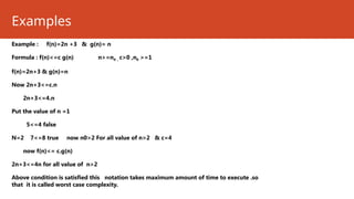
23. Examples
Example : f(n)=2n +3 & g(n)= n
Formula : f(n)<=c g(n) n>=n0 , c>0 ,n0 >=1
f(n)=2n+3 & g(n)=n
Now 2n+3<=c.n
2n+3<=4.n
Put the value of n =1
5<=4 false
N=2 7<=8 true now n0>2 For all value of n>2 & c=4
now f(n)<= c.g(n)
2n+3<=4n for all value of n>2
Above condition is satisfied this notation takes maximum amount of time to execute .so
that it is called worst case complexity.

24. • Big O notation describes an asymptotic upper bound on the growth rate of a function. While it is most
commonly used to express the worst-case time complexity of an algorithm, it can also be used to describe the
best-case time complexity in certain scenarios.
• Here's why and how:
• Big O as an Upper Bound: The fundamental definition of Big O, (f(n)=O(g(n))), means that for sufficiently
large (n), (f(n)) is bounded above by a constant multiple of (g(n)). This definition holds true regardless of
whether (f(n)) represents the worst-case, best-case, or average-case performance.
• Best Case with Big O: If an algorithm's best-case performance is, for example, constant time, one could
correctly state that its best-case time complexity is (O(1)). Similarly, if an algorithm has a best-case linear
time complexity, it could be described as (O(n)). Distinction from Omega and Theta: Big Omega ((
Omega )): notation is typically used to describe the asymptotic lower bound or the best-case complexity.
However, for a more precise description of the best case, especially when a tight bound is known, Big Omega (
(Omega )) or Big Theta ((Theta )) notation may be more appropriate.

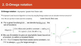
25. 2. Ω-Omega notation
Ω-Omega notation : Asymptotic “greater than”(faster rate).
 It represent Lower bound of algorithm run time. By using Big Omega notation we can calculate minimum amount of
time. We can say that it is best case time complexity. Lower bound, Best case

26. Example
Imagine you’re running a 100-meter race:
No matter how fast you are, you cannot complete it in less than 10 seconds (say).
So, Ω = 10 seconds (the best you can ever do).
But depending on obstacles, you might take up to 20 seconds (that’s the O(n) side).
Suppose we have a function that adds all numbers in an array:
int sum(int arr[], int n)
{ int total = 0;
for (int i = 0; i < n; i++)
{ total += arr[i]; }
return total; }
•Best case: Even if the array has easy numbers (like all zeros), we still have to check every element once.
•So, the time taken is at least proportional to n. Ω(n)

27. Example : f(n)=3n +2 g(n)=n
Formula : f(n)>=c g(n) n>=n0 , c>0 ,n0 >=1
f(n)=3n+2
3n+2>=1*n, c=1 put the value of n=1
n=1 5>=1 true n0>=1 for all value of n
It means that f(n)= Ω g(n).
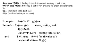
•Best case (Ω(1)): If the key is the first element, we only check once.
•Worst case (O(n)): If the key is last or not present, we check all n elements.
So:
•Ω(1) (minimum time, best case)
•O(n) (maximum time, worst case)

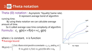
28. 3. -Theta notation

Theta (Θ) notation : Asymptotic “Equality”(same rate).
It represent average bond of algorithm
running time.
By using theta notation we can calculate average
amount of time.
So it called average case time complexity of algorithm.
Formula : c1 g(n)<=f(n)<=c2 g(n)
where c is constant, n is function
Average bound












0
2
1
0
2
1
all
for
)
(
)
(
)
(
c
0
s.t.
and
,
,
constants
positive
exist
there
:
)
(
))
(
(
n
n
n
g
c
n
f
n
g
n
c
c
n
f
n
g

29. Contd..
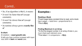
• So, if an algorithm is Θ(n²), it means:
• It won’t be faster than n² (except
constants).
• It won’t be slower than n² (except
constants).
• Its runtime always grows exactly like
n².
In short:
Θ notation = exact growth rate.
It tells you how runtime increases with input
size, both in best and worst case.
Examples:-
Reading a Book
•If each page takes constant time to read, and a book
has n pages total time = proportional to
→ n.
•This is Θ(n).
Finding Maximum in an Array
•To find the largest number in an array of size n, you
must check each element once.
•Time taken = n comparisons → Θ(n).

30. Numerical
Example 1: f(n)=5n+3 Example 2: f(n)=2n2+5n+10

31. Examples:-
Imagine a classroom of 100 students in which you gave your pen to one person. You
have to find that pen without knowing to whom you gave it.
Here are some ways to find the pen and what the O order is.
O(n2
): You go and ask the first person in the class if he has the pen. Also, you ask this person
about the other 99 people in the classroom if they have that pen and so on,
This is what we call O(n2
).
O(n): Going and asking each student individually is O(N).
O(log n): Now I divide the class into two groups, then ask: "Is it on the left side, or the right
side of the classroom?" Then I take that group and divide it into two and ask again, and so on.
Repeat the process till you are left with one student who has your pen. This is what you mean
by O(log n).

32. Properties of Asymptotic Notation
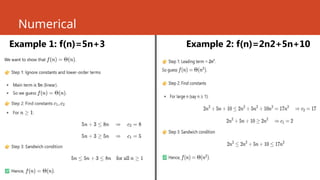
1. General Properties:
If f(n) is O(g(n)) then a*f(n) is also O(g(n)), where a is a constant.
Example:
f(n) = 5n²+5 is O(n²)
then, 2*f(n) = 2(5n²+5) = 10n²+10 is also O(n²).
Similarly, this property satisfies both Θ and Ω notation.
We can say,
If f(n) is Θ(g(n)) then a*f(n) is also Θ(g(n)), where a is a constant.
If f(n) is Ω (g(n)) then a*f(n) is also Ω (g(n)), where a is a constant.

33. Contd..
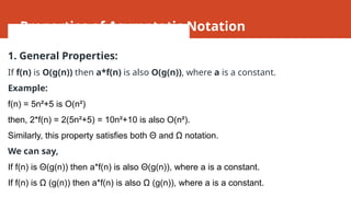
2. Transitive Properties:
If f(n) is O(g(n)) and g(n) is O(h(n)) then f(n) = O(h(n)).
Example:
If f(n) = n, g(n) = n² and h(n)=n³
n is O(n²) and n² is O(n³) then, n is O(n³)
Similarly, this property satisfies both Θ and Ω notation.
We can say,
If f(n) is Θ(g(n)) and g(n) is Θ(h(n)) then f(n) = Θ(h(n)) .
If f(n) is Ω (g(n)) and g(n) is Ω (h(n)) then f(n) = Ω (h(n))

34. Contd..
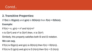
3. Reflexive Properties:
Reflexive properties are always easy to understand after transitive.
If f(n) is given then f(n) is O(f(n)). Since MAXIMUM VALUE OF f(n) will be f(n) ITSELF!
Hence x = f(n) and y = O(f(n) tie themselves in reflexive relation always.
Example:
f(n) = n² ; O(n²) i.e O(f(n))
Similarly, this property satisfies both Θ and Ω notation.
We can say that,
If f(n) is given then f(n) is Θ(f(n)).
If f(n) is given then f(n) is Ω (f(n)).

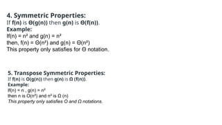
35. 4. Symmetric Properties:
If f(n) is Θ(g(n)) then g(n) is Θ(f(n)).
Example:
If(n) = n² and g(n) = n²
then, f(n) = Θ(n²) and g(n) = Θ(n²)
This property only satisfies for Θ notation.
5. Transpose Symmetric Properties:
If f(n) is O(g(n)) then g(n) is Ω (f(n)).
Example:
If(n) = n , g(n) = n²
then n is O(n²) and n² is Ω (n)
This property only satisfies O and Ω notations.

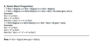
36. 6. Some More Properties:
1. If f(n) = O(g(n)) and f(n) = Ω(g(n)) then f(n) = Θ(g(n))
2. If f(n) = O(g(n)) and d(n)=O(e(n)) then f(n) + d(n) = O( max( g(n), e(n) ))
Example:
f(n) = n i.e O(n)
d(n) = n² i.e O(n²)
then f(n) + d(n) = n + n² i.e O(n²)
3. If f(n)=O(g(n)) and d(n)=O(e(n)) then f(n) * d(n) = O( g(n) * e(n))
Example:
f(n) = n i.e O(n)
d(n) = n² i.e O(n²)
then f(n) * d(n) = n * n² = n³ i.e O(n³)
______________________________________________________________________________
_
Note: If f(n) = O(g(n)) then g(n) = Ω(f(n))

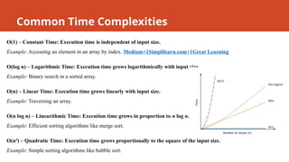
37. Common Time Complexities
O(1) – Constant Time: Execution time is independent of input size.
Example: Accessing an element in an array by index. Medium+1Simplilearn.com+1Great Learning
O(log n) – Logarithmic Time: Execution time grows logarithmically with input size.
Example: Binary search in a sorted array.
O(n) – Linear Time: Execution time grows linearly with input size.
Example: Traversing an array.
O(n log n) – Linearithmic Time: Execution time grows in proportion to n log n.
Example: Efficient sorting algorithms like merge sort.
O(n²) – Quadratic Time: Execution time grows proportionally to the square of the input size.
Example: Simple sorting algorithms like bubble sort.

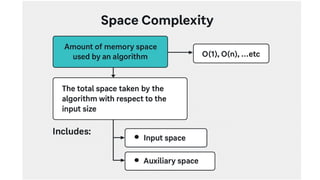
38. 2. Space Complexity
Space Complexity refers to the amount of memory (space) an algorithm needs to run,
based on the size of its input.
•Measures how much memory (RAM) an algorithm uses during execution.
•Includes:
•Memory for input
•Temporary variables
•Recursion stack (if applicable)
Example:
int arr[n]; // O(n) space

40. What It Includes:
Input space – memory used to store the input (not
always counted).
Auxiliary space – extra memory used by the
algorithm:
• Variables
• Arrays
• Stacks (especially in recursion)
• Buffers or caches
Space Complexity Notation:
Like time complexity, it is usually
expressed using Big O notation:
•O(1) → Constant space (very efficient)
•O(n) → Linear space (grows with input
size)
•O(n^2) → Quadratic space, etc.

41. Examples in C++
Example 1: Constant Space – O(1)
int sum(int a, int b)
{
int result = a + b; return result;
}
•Uses only a few variables → constant
space
Example 2: Linear Space – O(n)
void printArray(int arr[], int n)
{
for(int i = 0; i < n; i++)
{ cout << arr[i]; }
}
•Uses space for the input array: O(n)

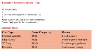
42. Example 3: Recursive Function – O(n)
int factorial(int n)
{
if (n == 0) return 1; return n * factorial(n - 1);
}
•Each recursive call adds a new frame to the stack.
•Needs O(n) space for the recursion stack.
Code Type Space Complexity Reason
Constant Variables O(1) Fixed memory
Single Array O(n) Memory grows with input
2D Array O(n²) Matrix or grid problems
Recursion O(n) Stack memory usage
Summary Table:

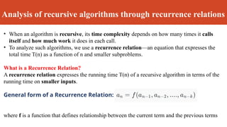
43. Analysis of recursive algorithms through recurrence relations
• When an algorithm is recursive, its time complexity depends on how many times it calls
itself and how much work it does in each call.
• To analyze such algorithms, we use a recurrence relation—an equation that expresses the
total time T(n) as a function of n and smaller subproblems.
What is a Recurrence Relation?
A recurrence relation expresses the running time T(n) of a recursive algorithm in terms of the
running time on smaller inputs.
General form of a Recurrence Relation:
where f is a function that defines relationship between the current term and the previous terms

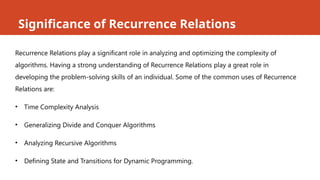
44. Significance of Recurrence Relations
Recurrence Relations play a significant role in analyzing and optimizing the complexity of
algorithms. Having a strong understanding of Recurrence Relations play a great role in
developing the problem-solving skills of an individual. Some of the common uses of Recurrence
Relations are:
• Time Complexity Analysis
• Generalizing Divide and Conquer Algorithms
• Analyzing Recursive Algorithms
• Defining State and Transitions for Dynamic Programming.

45. Types of Recurrence Relations:
1. Linear Recurrence Relation: In case of Linear Recurrence Relation every term
is dependent linearly on its previous term. Example of Linear Recurrence
Relation can be
T(n) = T(n-1) + T(n-2) + T(n-3)
2. Divide and Conquer Recurrence Relation: It the type of Recurrence Relation
which is obtained from Divide and Conquer Algorithm. Example of such
recurrence relation can be
T(n) = 3T(n/2) + 9n
3. First Order Recurrence Relation: It is the type of recurrence relation in which
every term is dependent on just previous term. Example of this type of
recurrence relation can be-
T(n) = T(n-1)2

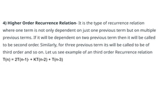
46. 4) Higher Order Recurrence Relation- It is the type of recurrence relation
where one term is not only dependent on just one previous term but on multiple
previous terms. If it will be dependent on two previous term then it will be called
to be second order. Similarly, for three previous term its will be called to be of
third order and so on. Let us see example of an third order Recurrence relation
T(n) = 2T(n-1)2
+ KT(n-2) + T(n-3)

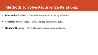
47. Methods to Solve Recurrence Relations:
• Substitution Method – Guess the answer and prove by induction.
• Recursion Tree Method – Draw the tree of recursive calls.
• Master’s Theorem – Direct shortcut to solve common forms.

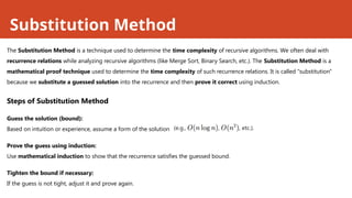
48. Substitution Method
The Substitution Method is a technique used to determine the time complexity of recursive algorithms. We often deal with
recurrence relations while analyzing recursive algorithms (like Merge Sort, Binary Search, etc.). The Substitution Method is a
mathematical proof technique used to determine the time complexity of such recurrence relations. It is called "substitution"
because we substitute a guessed solution into the recurrence and then prove it correct using induction.
Steps of Substitution Method
Guess the solution (bound):
Based on intuition or experience, assume a form of the solution
Prove the guess using induction:
Use mathematical induction to show that the recurrence satisfies the guessed bound.
Tighten the bound if necessary:
If the guess is not tight, adjust it and prove again.

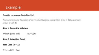
49. Example
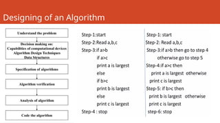
Consider recurrence: T(n)=T(n−1)+1
This recurrence means: the problem of size n is solved by solving a sub problem of size (n−1)plus a constant
amount of work (1).
Step 1: Guess the solution
We can guess that: T(n)=O(n)
Step 2: Induction Proof
Base Case (n = 1):
T(1)=1=O(1) True

50. Step 2: continued..
Step 3: Conclusion
Thus, T(n)=O(n)T(n) = O(n)T(n)=O(n)

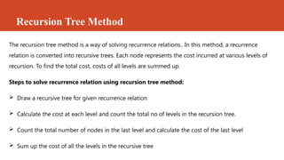
51. Recursion Tree Method
The recursion tree method is a way of solving recurrence relations.. In this method, a recurrence
relation is converted into recursive trees. Each node represents the cost incurred at various levels of
recursion. To find the total cost, costs of all levels are summed up.
Steps to solve recurrence relation using recursion tree method:
 Draw a recursive tree for given recurrence relation
 Calculate the cost at each level and count the total no of levels in the recursion tree.
 Count the total number of nodes in the last level and calculate the cost of the last level
 Sum up the cost of all the levels in the recursive tree

52. L2.52
Example of recursion tree
Solve T(n) = T(n/4) + T(n/2) + n2
:

53. L2.53
Example of recursion tree
T(n)
Solve T(n) = T(n/4) + T(n/2) + n2
:

54. L2.54
Example of recursion tree
T(n/4) T(n/2)
n2
Solve T(n) = T(n/4) + T(n/2) + n2
:

55. L2.55
Example of recursion tree
Solve T(n) = T(n/4) + T(n/2) + n2
:
n2
(n/4)2 (n/2)2
T(n/16) T(n/8) T(n/8) T(n/4)

56. L2.56
Example of recursion tree
(n/16)2
(n/8)2
(n/8)2
(n/4)2
(n/4)2 (n/2)2
Q(1)
…
Solve T(n) = T(n/4) + T(n/2) + n2
:
n2

57. L2.57
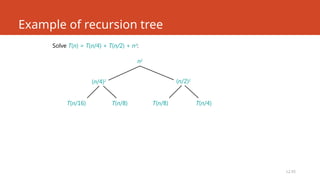
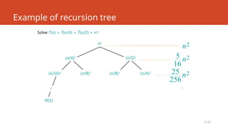
Example of recursion tree
Solve T(n) = T(n/4) + T(n/2) + n2
:
(n/16)2
(n/8)2
(n/8)2
(n/4)2
(n/4)2 (n/2)2
Q(1)
…
2
n
n2

58. L2.58
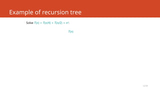
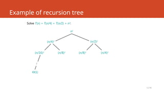
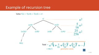
Example of recursion tree
Solve T(n) = T(n/4) + T(n/2) + n2
:
(n/16)2
(n/8)2
(n/8)2
(n/4)2
(n/4)2 (n/2)2
Q(1)
…
2
16
5 n
2
n
n2

59. L2.59
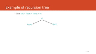
Example of recursion tree
Solve T(n) = T(n/4) + T(n/2) + n2
:
(n/16)2
(n/8)2
(n/8)2
(n/4)2
(n/4)2
Q(1)
…
2
16
5 n
2
n
2
256
25 n
n2
(n/2)2
…

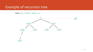
60. L2.60
Example of recursion tree
Solve T(n) = T(n/4) + T(n/2) + n2
:
(n/16)2
(n/8)2
(n/8)2
(n/4)2
(n/4)2
Q(1)
…
2
16
5 n
2
n
2
256
25 n
   
 
1
3
16
5
2
16
5
16
5
2





n
…
Total =
= Q(n2
)
n2
(n/2)2
geometric series

61. L2.61
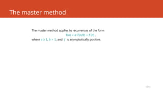
The master method
The master method applies to recurrences of the form
T(n) = a T(n/b) + f (n) ,
where a ³ 1, b > 1, and f is asymptotically positive.

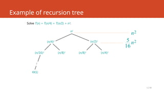
62. L2.62
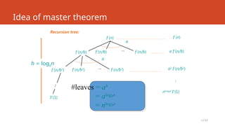
f (n/b)
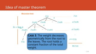
Idea of master theorem
f (n/b) f (n/b)
T (1)
…
Recursion tree:
…
f (n)
a
f (n/b2
)
f (n/b2
) f (n/b2
)
…
a
h = logbn
f (n)
a f (n/b)
a2
f (n/b2
)
…
#leaves = ah
= alogbn
= nlogba
nlogba
T (1)

63. L2.63
Three common cases
Compare f (n) with nlogba
:
1. f(n) = O(nlogba – e
) for some constant e > 0.
• f(n) grows polynomially slower than nlogba
(by an ne
factor).
Solution: T(n) = Q(nlogba
) .

64. L2.64
f (n/b)
Idea of master theorem
f (n/b) f (n/b)
T (1)
…
Recursion tree:
…
f (n)
a
f (n/b2
)
f (n/b2
) f (n/b2
)
…
a
h = logbn
f (n)
a f (n/b)
a2
f (n/b2
)
…
nlogba
T (1)
CASE 1: The weight increases
geometrically from the root to
the leaves. The leaves hold a
constant fraction of the total
weight.
Q(nlogba
)

65. L2.65
Three common cases
Compare f (n) with nlogba
:
2. f(n) = Q(nlogba
lgk
n) for some constant k ³ 0.
• f(n) and nlogba
grow at similar rates.
Solution: T(n) = Q(nlogba
lgk+1
n) .

66. L2.66
f (n/b)
Idea of master theorem
f (n/b) f (n/b)
T (1)
…
Recursion tree:
…
f (n)
a
f (n/b2
)
f (n/b2
) f (n/b2
)
…
a
h = logbn
f (n)
a f (n/b)
a2
f (n/b2
)
…
nlogba
T (1)
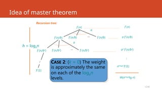
CASE 2: (k = 0) The weight
is approximately the same
on each of the logbn
levels. Q(nlogba
lg n)

67. L2.67
Three common cases (cont.)
Compare f (n) with nlogba
:
3. f(n) = W(nlogba + e
) for some constant e > 0.
• f(n) grows polynomially faster than nlogba
(by
an ne
factor),
and f(n) satisfies the regularity condition that
af(n/b) £ c f(n) for some constant c < 1.
Solution: T(n) = Q( f(n)) .

68. L2.68
f (n/b)
Idea of master theorem
f (n/b) f (n/b)
T (1)
…
Recursion tree:
…
f (n)
a
f (n/b2
)
f (n/b2
) f (n/b2
)
…
a
h = logbn
f (n)
a f (n/b)
a2
f (n/b2
)
…
nlogba
T (1)
CASE 3: The weight decreases
geometrically from the root to
the leaves. The root holds a
constant fraction of the total
weight.
Q( f (n))

69. L2.69
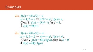
Examples
Ex. T(n) = 4T(n/2) + n
a = 4, b = 2  nlogba
= n2
; f(n) = n.
CASE 1: f(n) = O(n2 – e
) for e = 1.
 T(n) = Q(n2
).
Ex. T(n) = 4T(n/2) + n2
a = 4, b = 2  nlogba
= n2
; f(n) = n2
.
CASE 2: f(n) = Q(n2
lg0
n), that is, k = 0.
 T(n) = Q(n2
lgn).

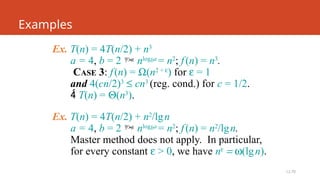
70. L2.70
Examples
Ex. T(n) = 4T(n/2) + n3
a = 4, b = 2  nlogba
= n2
; f(n) = n3
.
CASE 3: f(n) = W(n2 + e
) for e = 1
and 4(cn/2)3
£ cn3
(reg. cond.) for c = 1/2.
 T(n) = Q(n3
).
Ex. T(n) = 4T(n/2) + n2
/lgn
a = 4, b = 2  nlogba
= n2
; f(n) = n2
/lgn.
Master method does not apply. In particular,
for every constant e > 0, we have ne
= w(lgn).

71. Thank
you