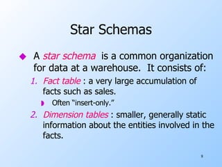
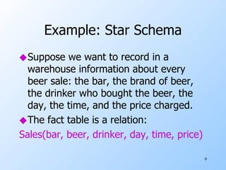
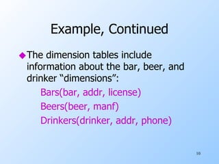
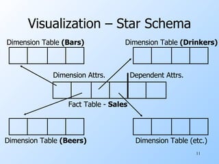
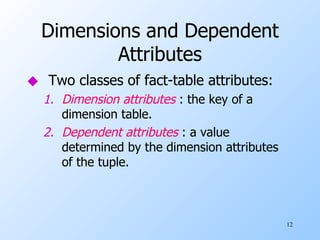
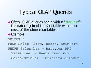
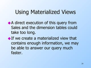
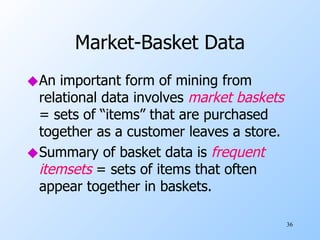
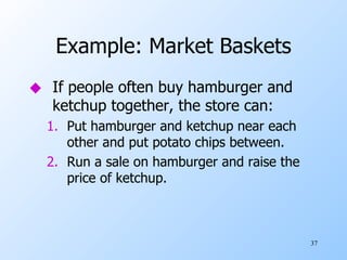
The document discusses various techniques for data warehousing and online analytical processing (OLAP), including constructing data warehouses, star schemas, materialized views, data cubes, and data mining. Specifically, it describes how a data warehouse can be used to integrate data from multiple sources and support complex OLAP queries run against historical data. It provides examples of star schemas, materialized views, data cubes, and market basket analysis to find frequent itemsets.

1. On-Line Application Processing Warehousing Data Cubes Data Mining

2. Overview Traditional database systems are tuned to many, small, simple queries. Some new applications use fewer, more time-consuming, complex queries. New architectures have been developed to handle complex “analytic” queries efficiently.

3. The Data Warehouse The most common form of data integration. Copy sources into a single DB ( warehouse ) and try to keep it up-to-date. Usual method: periodic reconstruction of the warehouse, perhaps overnight. Frequently essential for analytic queries.

4. OLTP Most database operations involve On-Line Transaction Processing (OTLP). Short, simple, frequent queries and/or modifications, each involving a small number of tuples. Examples: Answering queries from a Web interface, sales at cash registers, selling airline tickets.

5. OLAP Of increasing importance are On-Line Application Processing (OLAP) queries. Few, but complex queries --- may run for hours. Queries do not depend on having an absolutely up-to-date database.

6. OLAP Examples Amazon analyzes purchases by its customers to come up with an individual screen with products of likely interest to the customer. Analysts at Wal-Mart look for items with increasing sales in some region.

7. Common Architecture Databases at store branches handle OLTP. Local store databases copied to a central warehouse overnight. Analysts use the warehouse for OLAP.

8. Star Schemas A star schema is a common organization for data at a warehouse. It consists of: Fact table : a very large accumulation of facts such as sales. Often “insert-only.” Dimension tables : smaller, generally static information about the entities involved in the facts.

9. Example: Star Schema Suppose we want to record in a warehouse information about every beer sale: the bar, the brand of beer, the drinker who bought the beer, the day, the time, and the price charged. The fact table is a relation: Sales(bar, beer, drinker, day, time, price)

10. Example, Continued The dimension tables include information about the bar, beer, and drinker “dimensions”: Bars(bar, addr, license) Beers(beer, manf) Drinkers(drinker, addr, phone)

11. Visualization – Star Schema Dimension Table (Beers) Dimension Table (etc.) Dimension Table (Drinkers) Dimension Table (Bars) Fact Table - Sales Dimension Attrs. Dependent Attrs.

12. Dimensions and Dependent Attributes Two classes of fact-table attributes: Dimension attributes : the key of a dimension table. Dependent attributes : a value determined by the dimension attributes of the tuple.

13. Example: Dependent Attribute price is the dependent attribute of our example Sales relation. It is determined by the combination of dimension attributes: bar , beer , drinker , and the time (combination of day and time-of-day attributes).

14. Approaches to Building Warehouses ROLAP = “relational OLAP”: Tune a relational DBMS to support star schemas. MOLAP = “multidimensional OLAP”: Use a specialized DBMS with a model such as the “data cube.”

15. ROLAP Techniques Bitmap indexes : For each key value of a dimension table (e.g., each beer for relation Beers) create a bit-vector telling which tuples of the fact table have that value. Materialized views : Store the answers to several useful queries (views) in the warehouse itself.

16. Typical OLAP Queries Often, OLAP queries begin with a “ star join ”: the natural join of the fact table with all or most of the dimension tables. Example: SELECT * FROM Sales, Bars, Beers, Drinkers WHERE Sales.bar = Bars.bar AND Sales.beer = Beers.beer AND Sales.drinker = Drinkers.drinker;

17. Typical OLAP Queries --- (2) The typical OLAP query will: Start with a star join. Select for interesting tuples, based on dimension data. Group by one or more dimensions. Aggregate certain attributes of the result.

18. Example: OLAP Query For each bar in Palo Alto, find the total sale of each beer manufactured by Anheuser-Busch. Filter: addr = “Palo Alto” and manf = “Anheuser-Busch”. Grouping: by bar and beer . Aggregation: Sum of price .

19. Example: In SQL SELECT bar, beer, SUM(price) FROM Sales NATURAL JOIN Bars NATURAL JOIN Beers WHERE addr = ’Palo Alto’ AND manf = ’Anheuser-Busch’ GROUP BY bar, beer;

20. Using Materialized Views A direct execution of this query from Sales and the dimension tables could take too long. If we create a materialized view that contains enough information, we may be able to answer our query much faster.

21. Example: Materialized View Which views could help with our query? Key issues: It must join Sales , Bars , and Beers , at least. It must group by at least bar and beer . It must not select out Palo-Alto bars or Anheuser-Busch beers. It must not project out addr or manf .

22. Example --- Continued Here is a materialized view that could help: CREATE VIEW BABMS(bar, addr, beer, manf, sales) AS SELECT bar, addr, beer, manf, SUM(price) sales FROM Sales NATURAL JOIN Bars NATURAL JOIN Beers GROUP BY bar, addr, beer, manf; Since bar -> addr and beer -> manf, there is no real grouping. We need addr and manf in the SELECT.

23. Example --- Concluded Here’s our query using the materialized view BABMS: SELECT bar, beer, sales FROM BABMS WHERE addr = ’Palo Alto’ AND manf = ’Anheuser-Busch’;

24. MOLAP and Data Cubes Keys of dimension tables are the dimensions of a hypercube. Example: for the Sales data, the four dimensions are bar , beer , drinker , and time . Dependent attributes (e.g., price ) appear at the points of the cube.

25. Visualization - Data Cubes price bar beer drinker

26. Marginals The data cube also includes aggregation (typically SUM) along the margins of the cube. The marginals include aggregations over one dimension, two dimensions,…

27. Visualization - Data Cube w/ Aggregation price bar beer drinker SUM over all Drinkers

28. Example: Marginals Our 4-dimensional Sales cube includes the sum of price over each bar, each beer, each drinker, and each time unit (perhaps days). It would also have the sum of price over all bar-beer pairs, all bar-drinker-day triples,…

29. Structure of the Cube Think of each dimension as having an additional value *. A point with one or more *’s in its coordinates aggregates over the dimensions with the *’s. Example: Sales(“Joe’s Bar”, “Bud”, *, *) holds the sum over all drinkers and all time of the Bud consumed at Joe’s.

30. Drill-Down Drill-down = “de-aggregate” = break an aggregate into its constituents. Example : having determined that Joe’s Bar sells very few Anheuser-Busch beers, break down his sales by particular A.-B. beer.

31. Roll-Up Roll-up = aggregate along one or more dimensions. Example : given a table of how much Bud each drinker consumes at each bar, roll it up into a table giving total amount of Bud consumed for each drinker.

32. Roll Up and Drill Down $ of Anheuser-Busch by drinker/bar $ of A-B / drinker Roll up by Bar $ of A-B Beers / drinker Drill down by Beer 40 31 38 Blue Chalk 42 36 50 Nut- House 30 33 45 Joe’s Bar Mary Bob Jim 112 100 133 Mary Bob Jim 35 40 48 Bud Light 37 31 45 M’lob 40 29 40 Bud Mary Bob Jim

33. Materialized Data-Cube Views Data cubes invite materialized views that are aggregations in one or more dimensions. Dimensions may not be completely aggregated --- an option is to group by an attribute of the dimension table.

34. Example A materialized view for our Sales data cube might: Aggregate by drinker completely. Not aggregate at all by beer . Aggregate by time according to the week . Aggregate according to the city of the bar.

35. Data Mining Data mining is a popular term for queries that summarize big data sets in useful ways. Examples : Clustering all Web pages by topic. Finding characteristics of fraudulent credit-card use.

36. Market-Basket Data An important form of mining from relational data involves market baskets = sets of “items” that are purchased together as a customer leaves a store. Summary of basket data is frequent itemsets = sets of items that often appear together in baskets.

37. Example: Market Baskets If people often buy hamburger and ketchup together, the store can: Put hamburger and ketchup near each other and put potato chips between. Run a sale on hamburger and raise the price of ketchup.

38. Finding Frequent Pairs The simplest case is when we only want to find “frequent pairs” of items. Assume data is in a relation Baskets(basket, item) . The support threshold s is the minimum number of baskets in which a pair appears before we are interested.

39. Frequent Pairs in SQL SELECT b1.item, b2.item FROM Baskets b1, Baskets b2 WHERE b1.basket = b2.basket AND b1.item < b2.item GROUP BY b1.item, b2.item HAVING COUNT(*) >= s; Look for two Basket tuples with the same basket and different items. First item must precede second, so we don’t count the same pair twice. Create a group for each pair of items that appears in at least one basket. Throw away pairs of items that do not appear at least s times.

40. A-Priori Trick --- (1) Straightforward implementation involves a join of a huge Baskets relation with itself. The a-priori algorithm speeds the query by recognizing that a pair of items { i , j } cannot have support s unless both { i } and { j } do.

41. A-Priori Trick --- (2) Use a materialized view to hold only information about frequent items. INSERT INTO Baskets1(basket, item) SELECT * FROM Baskets WHERE item IN ( SELECT item FROM Baskets GROUP BY item HAVING COUNT(*) >= s ); Items that appear in at least s baskets.

42. A-Priori Algorithm Materialize the view Baskets1 . Run the obvious query, but on Baskets1 instead of Baskets . Computing Baskets1 is cheap, since it doesn’t involve a join. Baskets1 probably has many fewer tuples than Baskets . Running time shrinks with the square of the number of tuples involved in the join.

43. Example: A-Priori Suppose: A supermarket sells 10,000 items. The average basket has 10 items. The support threshold is 1% of the baskets. At most 1/10 of the items can be frequent. Probably , the minority of items in one basket are frequent -> factor 4 speedup.