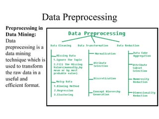
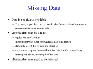
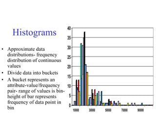
This document provides an overview of key concepts in data preprocessing for data science. It discusses why preprocessing is important due to issues with real-world data being dirty, incomplete, noisy or inconsistent. The major tasks covered are data cleaning (handling missing data, outliers, inconsistencies), data integration, transformation (normalization, aggregation), and reduction (discretization, dimensionality reduction). Clustering and regression techniques are also introduced for handling outliers and smoothing noisy data. The goal of preprocessing is to prepare raw data into a format suitable for analysis to obtain quality insights and predictions.

1. CD404- Introduction to Data Science
Data Collection strategies
Data Preprocessing

2. ETL (Extract, Transform, and Load)
Extract, Transform and Load is the technique of
extracting the record from sources (which is present
outside or on-premises, etc.) to a staging area, then
transforming or reformatting with business manipulation
performed on it in order to fit the operational needs or
data analysis, and later loading into the goal or
destination databases or data warehouse.

3. ETL v/s ELT

4. Types of Analytics
Descriptive Analytics –What happened?
Diagnostics Analytics – Why happened?
Predictive Analytics- What will happen?
Prescriptive Analytics – what should we do?

5. Data Collection
To analyze and make decisions about a certain business,
sales, etc., data will be collected. This collected data will
help in making some conclusions about the performance of a
particular business.
Thus, data collection is essential to analyze the performance
of a business unit, solving a problem and making
assumptions about specific things when required.

6. Data Science Process Model
Frame the problem – Objective to be identified
Collect the raw data needed for your problem
Process the data for analysis -EDA
Data Visualisation
Dimensionality Reduction
Model Building

7. Definition: In Statistics, data collection is a process of
gathering information from all the relevant sources to find a
solution to the research problem. Most of the organizations
use data collection methods to make assumptions about
future probabilities and trends.
Primary Data Collection methods
Secondary Data Collection methods

8. Primary data or raw data is a type of information that is obtained
directly from the first-hand source through experiments, surveys or
observations.
Quantitative Data Collection Methods
It is based on mathematical calculations using various formats and
statistical methods, mean, median or mode measures.
Qualitative Data Collection Methods
It does not involve any mathematical calculations. This method is
closely associated with elements that are not quantifiable. This
qualitative data collection method includes interviews,
questionnaires, observations, case studies, etc.

9. Secondary data is data collected by someone other than the
actual user. It means that the information is already available, and
someone analyses it. The secondary data includes magazines,
newspapers, books, journals, etc. It may be either published data
or unpublished data.
Published data are available in various resources including
Government publications
Public records
Historical and statistical documents
Business documents
Technical and trade journals
Data Repositories
Unpublished Data : Raw copy before publication

10. Outline
• Why data preprocessing?
• Data cleaning
• Data integration and transformation
• Data reduction
• Discretization and concept hierarchy generation
• Summary

11. Why Data Preprocessing?
• Data in the real world is dirty
– incomplete: lacking attribute values, lacking certain attributes
of interest, or containing only aggregate data
– noisy: containing errors or outliers
– inconsistent: containing discrepancies in codes or names
• No quality data, no quality mining results!
– Quality decisions must be based on quality data
– Data warehouse needs consistent integration of quality data

12. • A multi-dimensional measure of data quality:
– A well-accepted multi-dimensional view:
• accuracy, completeness, consistency,
timeliness, believability, value added,
interpretability, accessibility
– Broad categories:
• intrinsic, contextual, representational, and
accessibility.

13. Dirty Data
• incomplete
• noisy
• inconsistent
• No Quality Data
Multidimensional measure of quality of data
 Accuracy
 completeness
 consistency
 Timeliness
 Reliability
 Accessibility
 Interpretability

14. Major Tasks in Data Preprocessing
• Data cleaning
– Fill in missing values, smooth noisy data, identify or remove
outliers, and resolve inconsistencies
• Data integration
– Integration of multiple databases, data cubes, files, or notes
• Data transformation
– Normalization (scaling to a specific range)
– Aggregation

15. • Data reduction
– Obtains reduced representation in volume but
produces the same or similar analytical results
– Data discretization: with particular importance,
especially for numerical data
– Data aggregation, dimensionality reduction,
data compression,generalization
Forms of data preprocessing : Data cleaning or
transformation
diagrammatic representation on next slide
For ex. -2,32,100 ( single digit/2 digit/3 digit) transofrmed
into 0 to 1 scale, 0.02,0.32,1.0

17. Outline
• Why preprocess the data?
• Data cleaning
• Data integration and transformation
• Data reduction
• Discretization and concept hierarchy generation
• Summary

18. Data Cleaning
• Data cleaning tasks
– Fill in missing values
– Identify outliers and smooth out noisy data
– Correct inconsistent data

19. Missing Data
• Data is not always available
– E.g., many tuples have no recorded value for several attributes, such
as customer income in sales data
• Missing data may be due to
– equipment malfunction
– inconsistent with other recorded data and thus deleted
– data not entered due to misunderstanding
– certain data may not be considered important at the time of entry
– not register history or changes of the data
• Missing data may need to be inferred

20. Missing data
•Not availability of data
•Equipment malfunctioning
•Inconsistent, thus deleted
•Data not entered
•Certain data may not be important at the time of entry
How to handle missing data?
•Manually entry
•Attribute mean
•Standardization
•normalization

21. DataFrame : an object useful in representing data in form of
rows and columns.
Once data is stored in dataframe , we can perform operations to
analyse and understand data.
import pandas as pd
import xlrd
df= pd.read_excel(path, “Sheet1”)
df

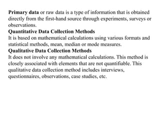
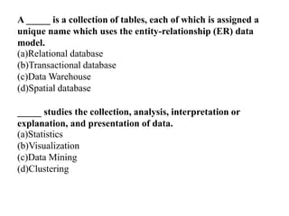
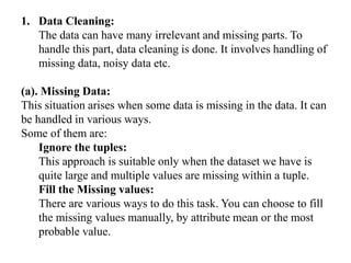
22. Sample Dataset
Countrydata=
[['India‘, 38.0, 68000.0] ,
['France‘, 43.0, 45000.0],
['Germany‘, 30.0, 54000.0],
['France' ,48.0,NaN]
]
List or tuple or dictionary
Df=pd.DataFrame(countrydata,
columns=[“country”,”no_states”,”Area”])

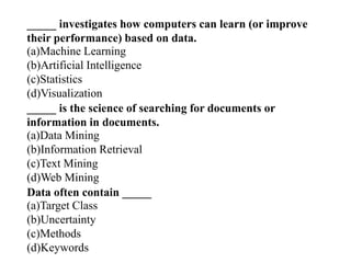
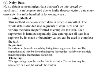
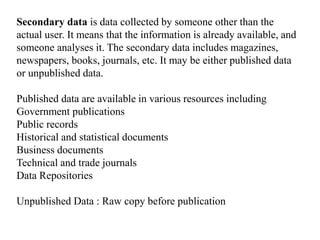
23. # importing libraries
import numpy as nm
import matplotlib.pyplot as mtp
import pandas as pd
#importing datasets
data_set= pd.read_csv('Dataset.csv')
#Viewing Dataframe , position index
x= data_set.iloc[:, [0:2]]
#Using column names
y= data_set.loc[:, [‘country’,’area’]]
'India‘, 38.0, 68000.0
'France‘, 43.0, 45000.0
’Germany‘, 30.0, 54000.0
’France' ,48.0,NaN
Country no_states area
0 India 38.0 68000.0
1
2
3

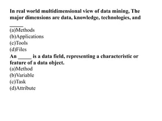
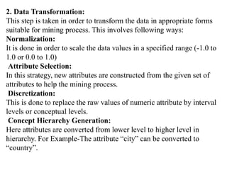
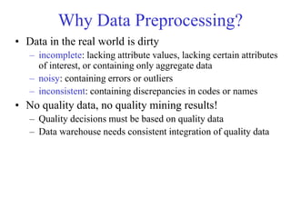
24. Operations
df.shape (rows,columns)
df.head(), df.head(2) default first 5 rows,
df.tail(), df.tail(4) default last 5 rows
df[2:5], df[0::2] intial,final,step value rows
df.columns Index[‘ ‘,’ ‘,’ ‘] column
names
df.empid or df[‘empid’] list of columns to be
passed

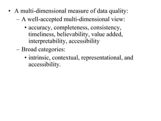
25. df[‘area’].min()
df[‘area’].max()
df.describe()
Count,mean,std,min,25%,50%,75%,max of all
coumns
df1=df.sort_values(‘country’)

26. variance measures variability from the average or
mean. It is calculated by taking the differences
between each number in the data set and the mean,
then squaring the differences to make them positive,
and finally dividing the sum of the squares by the
number of values in the data set.
Standard Deviation is square root of variance
measures

27. Missing data handling
df1=df.fillna(0)
df1=df.fillname({‘columnname’;value})
df1=df.dropna()

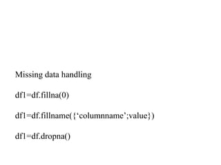
28. df.isnull().sum() ============= >zero initially
df[‘column’].mean()
df[‘column’].fillna(df[[‘column’].mean(), inplace=True)
df[‘column’].fillna(df[[‘column’].mode(), inplace=True)
df[‘column’].fillna(df[[‘column’].median(), inplace=True)
df.isnull().sum() ============= ==>zero

29. How to Handle Noisy Data?
• Binning method:
– first sort data and partition into (equi-depth) bins
– then one can smooth by bin means, smooth by bin median,
smooth by bin boundaries, etc.
– used also for discretization
• Clustering
– detect and remove outliers
• Semi-automated method: combined computer and
human inspection
– detect suspicious values and check manually
• Regression
– smooth by fitting the data into regression functions

30. Simple Discretization Methods: Binning
• Equal-width (distance) partitioning:
– It divides the range into N intervals of equal size: uniform
grid
– if A and B are the lowest and highest values of the attribute,
the width of intervals will be: W = (B-A)/N.
– The most straightforward
– But outliers may dominate presentation
– Skewed data is not handled well.
• Equal-depth (frequency) partitioning:
– It divides the range into N intervals, each containing
approximately same number of samples
– Good data scaling
– Managing categorical attributes can be tricky.

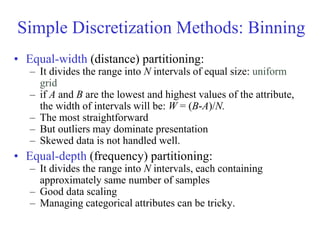
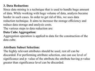
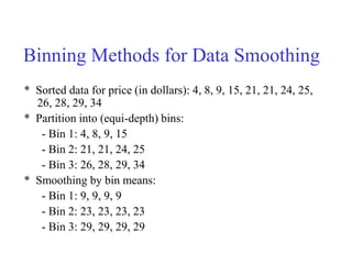
31. • Sorted data for price (in dollars): 4, 8, 9, 15,
21, 21, 24, 25, 26, 28, 29, 34
• Equal-width no of bins:3
• 34-4=30/3=10
• Bin 1: 4..4+10==4..14 [4,8,9]
• Bin 2:15..15+10==15..25 [15,21,21,24,25]
• Bin 3:26..26+10==26..36 [26,28,29,34]

32. Binning Methods for Data Smoothing
* Sorted data for price (in dollars): 4, 8, 9, 15, 21, 21, 24, 25,
26, 28, 29, 34
* Partition into (equi-depth) bins:
- Bin 1: 4, 8, 9, 15
- Bin 2: 21, 21, 24, 25
- Bin 3: 26, 28, 29, 34
* Smoothing by bin means:
- Bin 1: 9, 9, 9, 9
- Bin 2: 23, 23, 23, 23
- Bin 3: 29, 29, 29, 29

33. • Smoothing by bin median:
- Bin 1: 9 9, 9, 9
- Bin 2: 23, 23, 23, 23
- Bin 3: 29, 29, 29, 29
* Smoothing by bin boundaries: (closest boundary)
- Bin 1: 4, 4, 4, 15
- Bin 2: 21, 21, 25, 25
- Bin 3: 26, 26, 26, 34

34. Question
• Data:11,13,13,15,15,16,19,20,20,20,21,21,2
2,23,24,30,40,45,45,45,71,72,73,75
• Data:5, 10, 11, 13, 15, 35, 50, 55, 72, 92,
204, 215
• a) Smoothing by bin mean
• b) Smoothing by bin median
• c) Smoothing by bin boundaries
• Perform equal-width/equal-depth binning

35. • For the both methods, the best way of
determining k is by looking at the histogram
and try different intervals or groups.
Discretization
– reduce the number of values for a given continuous
attribute by dividing the range of the attribute into
intervals. Interval labels can then be used to replace
actual data values

36. Histograms
• Approximate data
distributions- frequency
distribution of continuous
values
• Divide data into buckets
• A bucket represents an
attribute-value/frequency
pair- range of values is bin-
height of bar represents
frequency of data point in
bin 0
5
10
15
20
25
30
35
40
10000 30000 50000 70000 90000

37. import numpy as np
import math
from sklearn.datasets import load_iris
# load iris data set
dataset = load_iris()
a = dataset.data
b = np.zeros(150)

38. # take 1st column among 4 column of data set
for i in range (150):
b[i]=a[i,1]
b=np.sort(b) #sort the array
• # create bins
• bin1=np.zeros((30,5))
• bin2=np.zeros((30,5))
• bin3=np.zeros((30,5))

39. # Bin mean
for i in range (0,150,5):
k=int(i/5)
mean=(b[i] + b[i+1] + b[i+2] + b[i+3] +
b[i+4])/5
for j in range(5):
bin1[k,j]=mean
print("Bin Mean: n",bin1)

40. Cluster Analysis

41. Select seed point randomly
Calculate distance of each point with seed ( called as centroid )
and form cluster with min. distance
Check the density and select new centroid
Formulate new clusters until optimality
Outlier points will be separated

42. Clustering
• Partition data set into clusters, and store cluster representation only
• Quality of clusters measured by their diameter (max distance
between any two objects in the cluster) or centroid distance (avg.
distance of each cluster object from its centroid)
• Can be very effective if data is clustered but not if data is “smeared”
• Can have hierarchical clustering (possibly stored in multi-
dimensional index tree structures (B+-tree, R-tree, quad-tree, etc))
• There are many choices of clustering definitions and clustering
algorithms

43. Outlier Treatment
Q1=df[‘area’].quantile(0.05)
Q2=df[‘area’].quantile(0.95)
df['a'] = np.where((df.a < Q1), Q1, df.a)
df.loc[(df.a > Q2), Q2, df.a)

44. Univariate outliers can be found when looking at a
distribution of values in a single feature space.
Multivariate outliers can be found in an n-
dimensional space (of n-features).
Point outliers are single data points that lay far from
the rest of the distribution.
Contextual outliers can be noise in data, such as
punctuation symbols when realizing text analysis
Collective outliers can be subsets of novelties in
data
[1,35,20,32,40,46,45,4500]

45. Regression
x
y
y = x + 1
X1
Y1
Y1’
•Linear regression (best line to fit
two variables)
•Multiple linear regression (more
than two variables, fit to a
multidimensional surface

46. Regression and Log-Linear Models
• Linear regression: Data are modeled to fit a straight
line:
– Often uses the least-square method to fit the line
• Multiple regression: allows a response variable y to
be modeled as a linear function of multidimensional
feature vector (predictor variables)
• Log-linear model: approximates discrete
multidimensional joint probability distributions

47. • Linear regression: Y =  +  X
– Two parameters ,  and  specify the line and are to be
estimated by using the data at hand.
– using the least squares criterion to the known values of Y1,
Y2, …, X1, X2, ….
• Multiple regression: Y = b0 + b1 X1 + b2 X2.
– Many nonlinear functions can be transformed into the above.
• Log-linear models:
– The multi-way table of joint probabilities is approximated by
a product of lower-order tables.
– Probability: p(a, b, c, d) = ab acad bcd
Regression Analysis and Log-Linear Models

48. Summary
• Data preparation is a big issue for both warehousing
and mining
• Data preparation includes
– Data cleaning and data integration
– Data reduction and feature selection
– Discretization
• A lot a methods have been developed but still an
active area of research

49. Numericals
1.Calculate variance and standard deviation for the
following data:
x 2,4,6,8,10
f 3,5,9,5,3
Ans: mean 6,var 5.44, std dev 2.33
2. Marks obtained by 5 students are 15,18,12,19 and 11.
Calculate std deviation, and variance
3. Calculate median 6, 2, 7, 9, 4, 1
4, 89, 65, 11, 54, 11, 90, 56,34

50. References
Data Preprocessing in Data Mining
Salvador García, Julián Luengo, Francisco Herrera (Springer)

51. MCQs
To remove noise and inconsistent data ____ is needed.
(a)Data Cleaning
(b)Data Transformation
(c)Data Reduction
(d)Data Integration
Multiple data sources may be combined is called as _____
(a)Data Reduction
(b)Data Cleaning
(c)Data Integration
(d)Data Transformation

52. A _____ is a collection of tables, each of which is assigned a
unique name which uses the entity-relationship (ER) data
model.
(a)Relational database
(b)Transactional database
(c)Data Warehouse
(d)Spatial database
_____ studies the collection, analysis, interpretation or
explanation, and presentation of data.
(a)Statistics
(b)Visualization
(c)Data Mining
(d)Clustering

53. _____ investigates how computers can learn (or improve
their performance) based on data.
(a)Machine Learning
(b)Artificial Intelligence
(c)Statistics
(d)Visualization
_____ is the science of searching for documents or
information in documents.
(a)Data Mining
(b)Information Retrieval
(c)Text Mining
(d)Web Mining
Data often contain _____
(a)Target Class
(b)Uncertainty
(c)Methods
(d)Keywords

54. In real world multidimensional view of data mining, The
major dimensions are data, knowledge, technologies, and
_____
(a)Methods
(b)Applications
(c)Tools
(d)Files
An _____ is a data field, representing a characteristic or
feature of a data object.
(a)Method
(b)Variable
(c)Task
(d)Attribute

55. The values of a _____ attribute are symbols or names of
things.
(a)Ordinal
(b)Nominal
(c)Ratio
(d)Interval
“Data about data” is referred to as _____
(a)Information
(b)Database
(c)Metadata
(d)File
______ partitions the objects into different groups.
(a)Mapping
(b)Clustering
(c)Classification
(d)Prediction

56. In _____, the attribute data are scaled so as to fall
within a smaller range, such as -1.0 to 1.0, or 0.0 to 1.0.
(a)Aggregation
(b)Binning
(c)Clustering
(d)Normalization
Normalization by ______ normalizes by moving the
decimal point of values of attributes.
(a)Z-Score
(b)Z-Index
(c)Decimal Scaling
(d)Min-Max Normalization
Used to transform the raw data in a useful and efficient
format.
a)Data Preparation
(b)Data Transformation
(c)Clustering
(d)Normalization

57. _______ is a top-down splitting technique based on a
specified number of bins.
(a)Normalization
(b)Binning
(c)Clustering
(d)Classification
Cluster Is
(a) A cluster is a subset of similar objects
(b) A subset of objects such that the distance between any of
the two objects in the cluster is less than the distance
between any object in the cluster and any object that is not
located inside it.
(c) A connected region of a multidimensional space with a
comparatively high density of objects.
(d) All of these

58. Data Preprocessing
Preprocessing in
Data Mining:
Data
preprocessing is a
data mining
technique which is
used to transform
the raw data in a
useful and
efficient format.

59. 1. Data Cleaning:
The data can have many irrelevant and missing parts. To
handle this part, data cleaning is done. It involves handling of
missing data, noisy data etc.
(a). Missing Data:
This situation arises when some data is missing in the data. It can
be handled in various ways.
Some of them are:
Ignore the tuples:
This approach is suitable only when the dataset we have is
quite large and multiple values are missing within a tuple.
Fill the Missing values:
There are various ways to do this task. You can choose to fill
the missing values manually, by attribute mean or the most
probable value.

60. (b). Noisy Data:
Noisy data is a meaningless data that can’t be interpreted by
machines. It can be generated due to faulty data collection, data entry
errors etc. It can be handled in following ways :
Binning Method:
This method works on sorted data in order to smooth it. The
whole data is divided into segments of equal size and then
various methods are performed to complete the task. Each
segmented is handled separately. One can replace all data in a
segment by its mean or boundary values can be used to complete
the task.
Regression:
Here data can be made smooth by fitting it to a regression function.The
regression used may be linear (having one independent variable) or multiple
(having multiple independent variables).
Clustering:
This approach groups the similar data in a cluster. The outliers may be
undetected or it will fall outside the clusters.

61. 2. Data Transformation:
This step is taken in order to transform the data in appropriate forms
suitable for mining process. This involves following ways:
Normalization:
It is done in order to scale the data values in a specified range (-1.0 to
1.0 or 0.0 to 1.0)
Attribute Selection:
In this strategy, new attributes are constructed from the given set of
attributes to help the mining process.
Discretization:
This is done to replace the raw values of numeric attribute by interval
levels or conceptual levels.
Concept Hierarchy Generation:
Here attributes are converted from lower level to higher level in
hierarchy. For Example-The attribute “city” can be converted to
“country”.

62. 3. Data Reduction:
Since data mining is a technique that is used to handle huge amount
of data. While working with huge volume of data, analysis became
harder in such cases. In order to get rid of this, we uses data
reduction technique. It aims to increase the storage efficiency and
reduce data storage and analysis costs.
The various steps to data reduction are:
Data Cube Aggregation:
Aggregation operation is applied to data for the construction of the
data cube.
Attribute Subset Selection:
The highly relevant attributes should be used, rest all can be
discarded. For performing attribute selection, one can use level of
significance and p- value of the attribute.the attribute having p-value
greater than significance level can be discarded.

63. Numerosity Reduction:
This enable to store the model of data instead of whole data, for
example: Regression Models.
Dimensionality Reduction:
This reduce the size of data by encoding mechanisms.It can be
lossy or lossless. If after reconstruction from compressed data,
original data can be retrieved, such reduction are called lossless
reduction else it is called lossy reduction. The two effective
methods of dimensionality reduction are:Wavelet transforms and
PCA (Principal Component Analysis).

64. Wavelet Transforms
The general procedure for applying a discrete wavelet
transform uses a hierarchical pyramid algorithm that halves
the data in each iteration, resulting in fast computational
speed. The method is as follows:
Take input data vector of the length, L (integer power of 2)
The two functions : sum or weighted average and weighted
difference are applied to pairs of input data, resulting in two
sets of data of length L/2
The two functions are recursively applied to sets of data
obtained in the previous loop, until the resulting data sets
obtained are of length 2.

65. Sampling
Sampling can be used as a data reduction technique since it allows a larger
data set to be represented by a much smaller random (or subset) of the
data. Suppose a large data set D, contains N tuples some of the possible
samples for D are:
• Simple random sample without replacement of size n: This created by
drawing n of the N tuples from D (n<N) where the probability of drawing
any tuple in D is I/N, that is all the tuples are equally likely.
•Simple random sample with replacement of size n: This is similar to the
above except that each time a tuple is drawn from D, it is recorded and
then replaced. That is after a tuple is drawn, it is placed back in D so that it
could be drawn again.
•Cluster sample: If the tuples in D are grouped into M mutually
disjount”clusters”then a simple random sample of m clusters can be
obtained, where m<M
•Stratified sample: If D is divided into mutually disjoint parts called strata,
a stratified random sample is obtained by simple random sample at each
stratum