Downloaded 11 times


![List comprehension
for(x in d)
for(y in d[x])
if(d[x,y]>100) ...
• vs
d[d > 100]](https://image.slidesharecdn.com/introductiontor-150424145149-conversion-gate02/75/Introduction-to-R-6-2048.jpg)
![Working with Data
csv <- read.csv(csv, header=F)
csv
names(csv) <- c(“orange”,”apple”)
•Data frames:
csv$bm
csv[1]](https://image.slidesharecdn.com/introductiontor-150424145149-conversion-gate02/75/Introduction-to-R-8-2048.jpg)
![Filtering Data
csv = csv[csv$Cha>100,]
or
subset(impressions, impressions$placement_id = 3599)
or
impressions$good = impressions$placement_id==3599
na.omit(impressions$good)](https://image.slidesharecdn.com/introductiontor-150424145149-conversion-gate02/75/Introduction-to-R-9-2048.jpg)
![Reading data
# read the data from csv
data = read.csv('data.csv', header = F, sep = 't', col.names = c('title',
'count'))
# order the data
data = data[order(data$count, decreasing=T),]
data$title = factor(data$title, levels=unique(as.character(data$title)))
head(data)
qplot(count, title, data=data)
# the other way around
qplot(title, count, data=data)](https://image.slidesharecdn.com/introductiontor-150424145149-conversion-gate02/75/Introduction-to-R-19-2048.jpg)
![Random Forest
> rf = randomForest(factor(Species) ~ Sepal.Length + Sepal.Width +
Petal.Length + Petal.Width, data =iris)
> rf$confusion
setosa versicolor virginica class.error
setosa 50 0 0 0.00
versicolor 0 47 3 0.06
virginica 0 4 46 0.08
> set.seed(1)
> iris.rf <- randomForest(iris[,-5], iris[,5], proximity=TRUE)
> plot(outlier(iris.rf), type="h",
> col=c("red", "green", "blue")[as.numeric(iris$Species)])](https://image.slidesharecdn.com/introductiontor-150424145149-conversion-gate02/75/Introduction-to-R-24-2048.jpg)
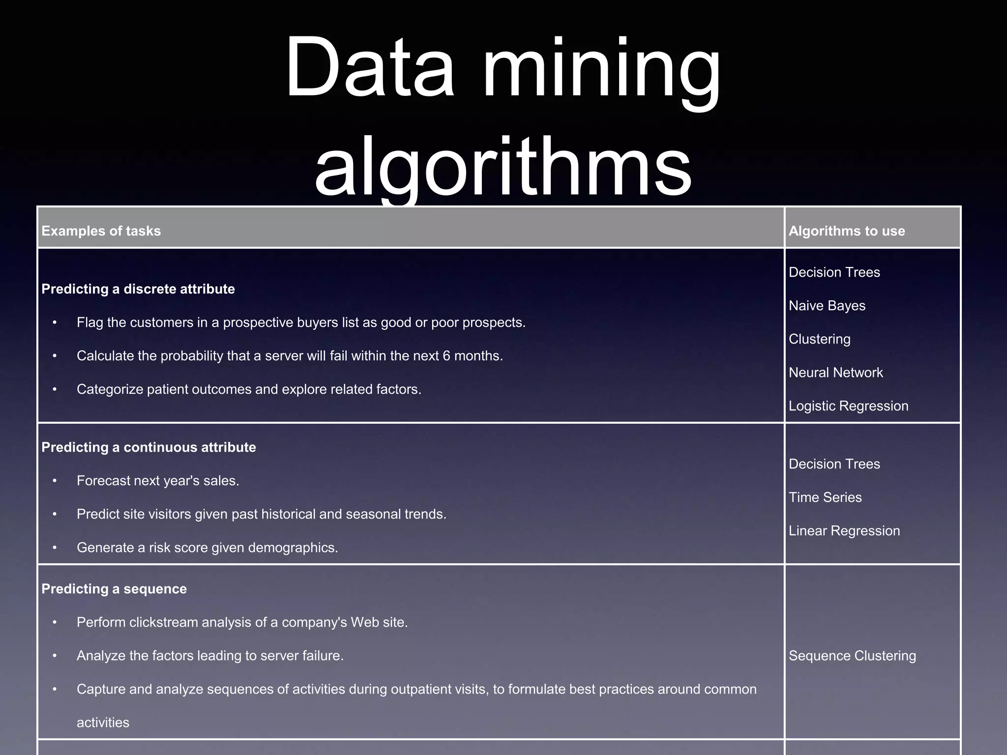

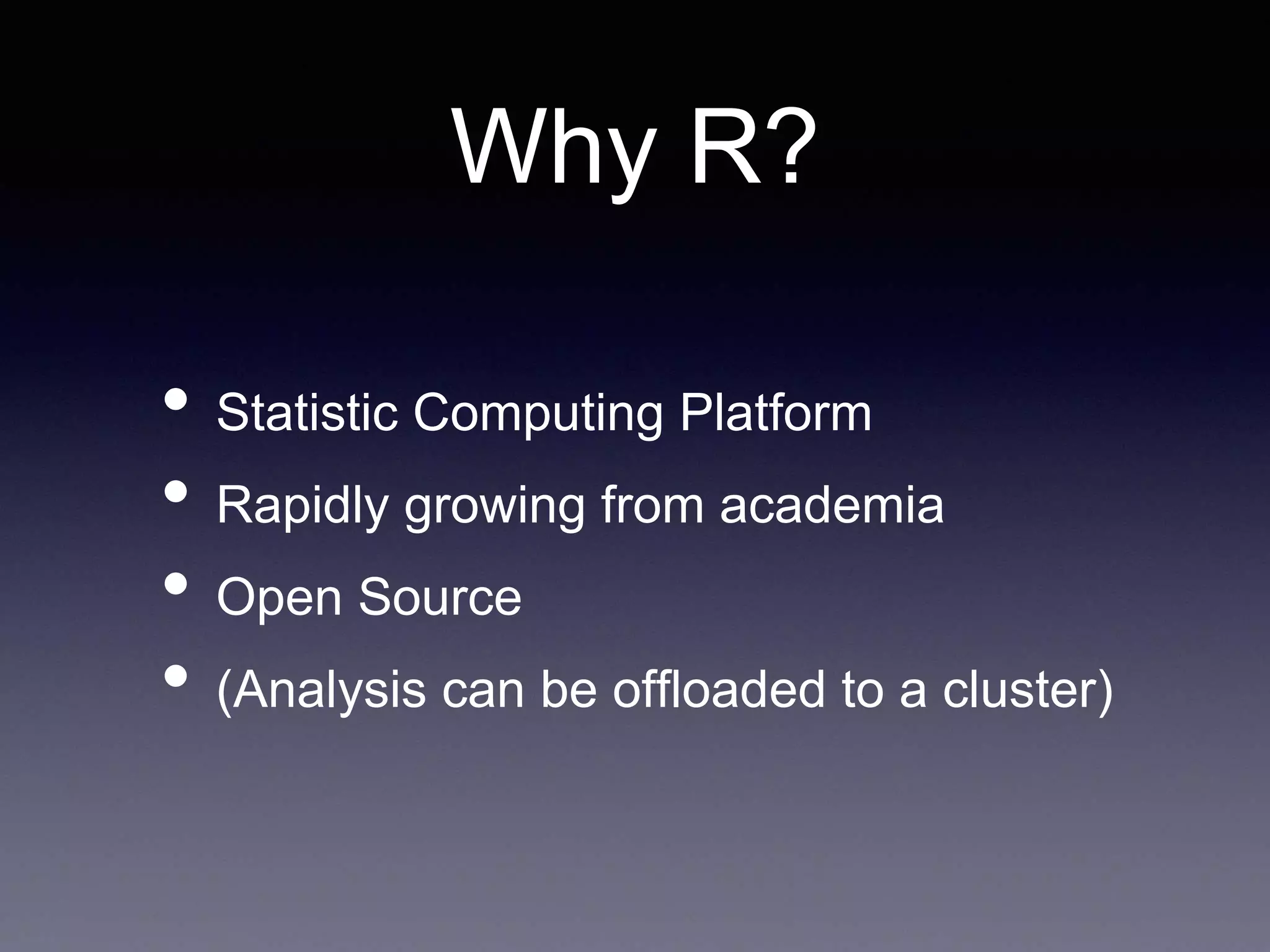
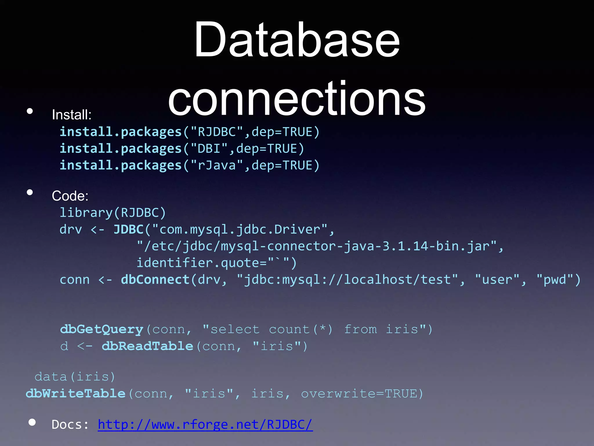
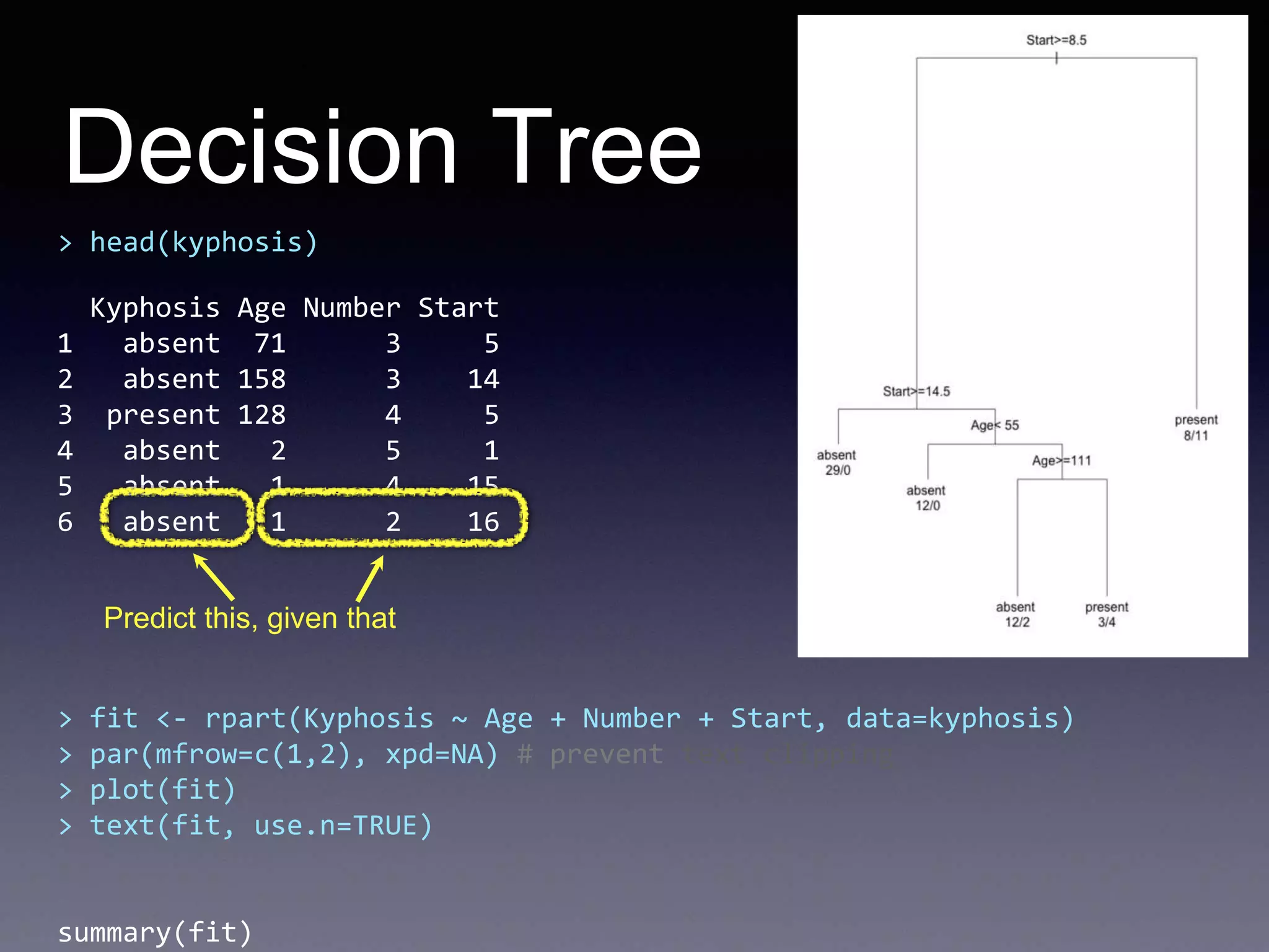
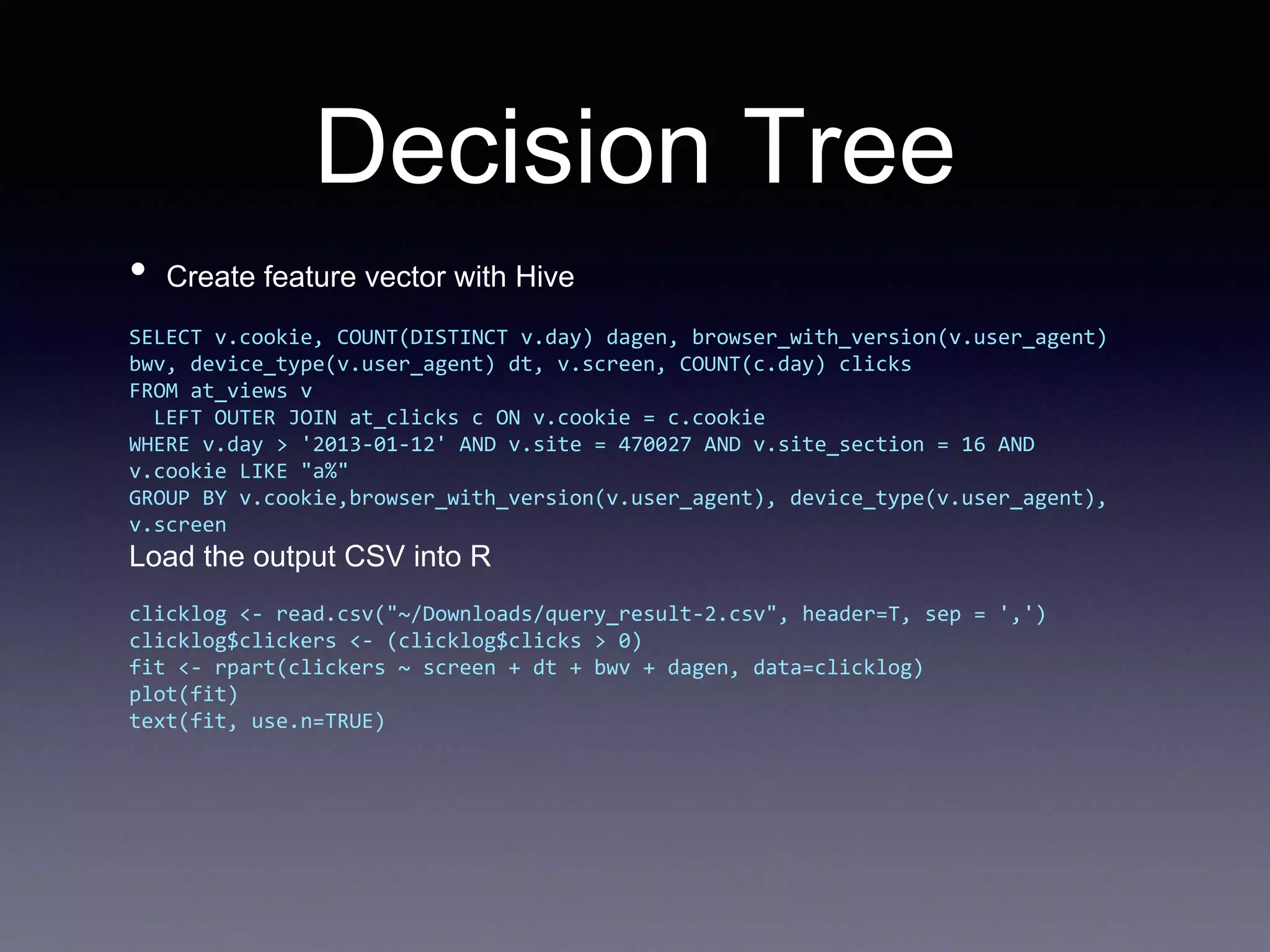
R is an open source statistical computing platform that is rapidly growing in popularity within academia. It allows for statistical analysis and data visualization. The document provides an introduction to basic R functions and syntax for assigning values, working with data frames, filtering data, plotting, and connecting to databases. More advanced techniques demonstrated include decision trees, random forests, and other data mining algorithms.


![Some R Examples[R table and Graphics] -Advanced Data Visualization in R (Some...](https://cdn.slidesharecdn.com/ss_thumbnails/exampless-160922204223-thumbnail.jpg?width=640&height=640&fit=bounds)