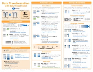
Grouped data frames allow dplyr functions to manipulate each group separately. The group_by() function creates a grouped data frame, while ungroup() removes grouping. Summarise() applies summary functions to columns to create a new table, such as mean() or count(). Join functions combine tables by matching values. Left, right, inner, and full joins retain different combinations of values from the tables.

1. Group Cases
group_by(.data, ..., add = FALSE)
Returns copy of table grouped by …
g_iris <- group_by(iris, Species)
ungroup(x, ...)
Returns ungrouped copy of table.
ungroup(g_iris)
wwwwww
www
Use group_by() to created a "grouped" copy of a table. dplyr
functions will manipulate each "group" separately and then
combine the results.
mtcars %>%
group_by(cyl) %>%
summarise(avg = mean(mpg))
Summarise Cases
These apply summary functions to
columns to create a new table.
Summary functions take vectors as
input and return one value (see back).
summary
function
Variations
• summarise_all() - Apply funs to every column.
• summarise_at() - Apply funs to specific columns.
• summarise_if() - Apply funs to all cols of one type.
www
www
summarise(.data, …)
Compute table of summaries. Also
summarise_().
summarise(mtcars, avg = mean(mpg))
count(x, ..., wt = NULL, sort = FALSE)
Count number of rows in each group defined
by the variables in … Also tally().
count(iris, Species)
Manipulate Cases
RStudio® is a trademark of RStudio, Inc. • CC BY RStudio • info@rstudio.com • 844-448-1212 • rstudio.com Learn more with browseVignettes(package = c("dplyr", "tibble")) • dplyr 0.5.0 • tibble 1.2.0 • Updated: 2017-01
Extract Cases
Add Cases
Arrange Cases
filter(.data, …)
Extract rows that meet logical criteria. Also
filter_(). filter(iris, Sepal.Length > 7)
distinct(.data, ..., .keep_all = FALSE)
Remove rows with duplicate values. Also
distinct_(). distinct(iris, Species)
sample_frac(tbl, size = 1, replace = FALSE,
weight = NULL, .env = parent.frame())
Randomly select fraction of rows.
sample_frac(iris, 0.5, replace = TRUE)
sample_n(tbl, size, replace = FALSE,
weight = NULL, .env = parent.frame())
Randomly select size rows.
sample_n(iris, 10, replace = TRUE)
slice(.data, …)
Select rows by position. Also slice_().
slice(iris, 10:15)
top_n(x, n, wt)
Select and order top n entries (by group if
grouped data). top_n(iris, 5, Sepal.Width)
Row functions return a subset of rows as a new table. Use a variant
that ends in _ for non-standard evaluation friendly code.
wwwwww
wwwwww
wwwwww
wwwwww
Logical and boolean operators to use with filter()
See ?base::logic and ?Comparison for help.
> >= !is.na() ! &
< <= is.na() %in% | xor()
wwwwww
arrange(.data, ...)
Order rows by values of a column (low to high),
use with desc() to order from high to low.
arrange(mtcars, mpg)
arrange(mtcars, desc(mpg))
wwwwww
add_row(.data, ..., .before = NULL,
.after = NULL)
Add one or more rows to a table.
add_row(faithful, eruptions = 1, waiting = 1)
Manipulate Variables
Extract Variables
Make New Variables
wwww
www ww
Column functions return a set of columns as a new table. Use a
variant that ends in _ for non-standard evaluation friendly code.
vectorized
function
These apply vectorized functions to
columns. Vectorized funs take vectors
as input and return vectors of the
same length as output (see back).
Data Transformation
with dplyr Cheat Sheet
wwwwww
www
wwww
mutate(.data, …)
Compute new column(s).
mutate(mtcars, gpm = 1/mpg)
transmute(.data, …)
Compute new column(s), drop others.
transmute(mtcars, gpm = 1/mpg)
mutate_all(.tbl, .funs, ...)
Apply funs to every column. Use with
funs(). mutate_all(faithful, funs(log(.),
log2(.)))
mutate_at(.tbl, .cols, .funs, ...)
Apply funs to specific columns. Use with
funs(), vars() and the helper functions for
select().
mutate_at(iris, vars( -Species), funs(log(.)))
mutate_if(.tbl, .predicate, .funs, ...)
Apply funs to all columns of one type. Use
with funs().
mutate_if(iris, is.numeric, funs(log(.)))
add_column(.data, ..., .before =
NULL, .after = NULL)
Add new column(s).
add_column(mtcars, new = 1:32)
rename(.data, …)
Rename columns.
rename(iris, Length = Sepal.Length)
w ww
Use these helpers with select(),
e.g. select(iris, starts_with("Sepal"))
contains(match)
ends_with(match)
matches(match)
:, e.g. mpg:cyl
-, e.g, -Species
Each observation, or
case, is in its own row
A B C
Each variable is
in its own column
A B C
&
dplyr functions work with pipes and expect tidy data. In tidy data:
pipes
x %>% f(y)
becomes f(x, y) num_range(prefix, range)
one_of(…)
starts_with(match)
select(.data, …)
Extract columns by name. Also select_if()
select(iris, Sepal.Length, Species)
wwwwww

2. C A B
1 a t
2 b u
3 c v
1 a t
2 b u
3 c v
C A B
A B C
a t 1
b u 2
c v 3
1 a t
2 b u
3 c v
C A B
A.x B.x C A.y B.y
a t 1 d w
b u 2 b u
c v 3 a t
a t 1 d w
b u 2 b u
c v 3 a t
A1 B1 C A2 B2
A B.x C B.y D
a t 1 t 3
b u 2 u 2
c v 3 NA NA
A B D
a t 3
b u 2
d w 1
A B C D
a t 1 3
b u 2 2
c v 3 NA
d w NA 1
A B C D
a t 1 3
b u 2 2
a t 1 3
b u 2 2
d w NA 1
A B C D
A B C D
a t 1 3
b u 2 2
c v 3 NA
A B C A B D
a t 1 a t 3
b u 2 b u 2
c v 3 d w 1
A B C
c v 3
A B C
a t 1
b u 2
A B C
a t 1
b u 2
a t 1
b u 2
A B C
c v 3
d w 4
A B C
c v 3
DF A B C
x a t 1
x b u 2
x c v 3
z c v 3
z d w 4
Counts
dplyr::n() - number of values/rows
dplyr::n_distinct() - # of uniques
sum(!is.na()) - # of non-NA’s
Location
mean() - mean, also mean(!is.na())
median() - median
Logicals
mean() - Proportion of TRUE’s
sum() - # of TRUE’s
Position/Order
dplyr::first() - first value
dplyr::last() - last value
dplyr::nth() - value in nth location of vector
Rank
quantile() - nth quantile
min() - minimum value
max() - maximum value
Spread
IQR() - Inter-Quartile Range
mad() - mean absolute deviation
sd() - standard deviation
var() - variance
Offsets
dplyr::lag() - Offset elements by 1
dplyr::lead() - Offset elements by -1
Cumulative Aggregates
dplyr::cumall() - Cumulative all()
dplyr::cumany() - Cumulative any()
cummax() - Cumulative max()
dplyr::cummean() - Cumulative mean()
cummin() - Cumulative min()
cumprod() - Cumulative prod()
cumsum() - Cumulative sum()
Rankings
dplyr::cume_dist() - Proportion of all values <=
dplyr::dense_rank() - rank with ties = min, no
gaps
dplyr::min_rank() - rank with ties = min
dplyr::ntile() - bins into n bins
dplyr::percent_rank() - min_rank scaled to [0,1]
dplyr::row_number() - rank with ties = "first"
Math
+, - , *, /, ^, %/%, %% - arithmetic ops
log(), log2(), log10() - logs
<, <=, >, >=, !=, == - logical comparisons
Misc
dplyr::between() - x >= left & x <= right
dplyr::case_when() - multi-case if_else()
dplyr::coalesce() - first non-NA values by
element across a set of vectors
dplyr::if_else() - element-wise if() + else()
dplyr::na_if() - replace specific values with NA
pmax() - element-wise max()
pmin() - element-wise min()
dplyr::recode() - Vectorized switch()
dplyr::recode_factor() - Vectorized switch() for
factors
Summary FunctionsVectorized Functions Combine Tables
RStudio® is a trademark of RStudio, Inc. • CC BY RStudio • info@rstudio.com • 844-448-1212 • rstudio.com Learn more with browseVignettes(package = c("dplyr", "tibble")) • dplyr 0.5.0 • tibble 1.2.0 • Updated: 2017-01
Combine Variables
bind_cols(…)
Returns tables placed side by
side as a single table.
BE SURE THAT ROWS ALIGN.
left_join(x, y, by = NULL,
copy=FALSE, suffix=c(“.x”,“.y”),…)
Join matching values from y to x.
right_join(x, y, by = NULL, copy =
FALSE, suffix=c(“.x”,“.y”),…)
Join matching values from x to y.
inner_join(x, y, by = NULL, copy =
FALSE, suffix=c(“.x”,“.y”),…)
Join data. Retain only rows with
matches.
full_join(x, y, by = NULL,
copy=FALSE, suffix=c(“.x”,“.y”),…)
Join data. Retain all values, all
rows.
Use a "Mutating Join" to join one table to columns
from another, matching values with the rows that
they correspond to. Each join retains a different
combination of values from the tables.
Use by = c("col1", "col2") to
specify the column(s) to match
on.
left_join(x, y, by = "A")
Use a named vector, by =
c("col1" = "col2"), to match on
columns with different names in
each data set.
left_join(x, y, by = c("C" = "D"))
Use suffix to specify suffix to give
to duplicate column names.
left_join(x, y, by = c("C" = "D"),
suffix = c("1", "2"))
Use bind_cols() to paste tables beside each other
as they are.
A B C
a t 1
b u 2
c v 3
+ =
x y
A B D
a t 3
b u 2
d w 1
Combine Cases
A B C
a t 1
b u 2
Use bind_rows() to paste tables below each other as
they are.
bind_rows(…, .id = NULL)
Returns tables one on top of the other
as a single table. Set .id to a column
name to add a column of the original
table names (as pictured)
intersect(x, y, …)
Rows that appear in both x and z.
setdiff(x, y, …)
Rows that appear in x but not z.
union(x, y, …)
Rows that appear in x or z. (Duplicates
removed). union_all() retains
duplicates.
Extract Rows
Use a "Filtering Join" to filter one table against the
rows of another.
semi_join(x, y, by = NULL, …)
Return rows of x that have a match in y.
USEFUL TO SEE WHAT WILL BE JOINED.
anti_join(x, y, by = NULL, …)
Return rows of x that do not have a
match in y. USEFUL TO SEE WHAT WILL
NOT BE JOINED.
A B C
a t 1
b u 2
c v 3
+
x
z
A B C
c v 3
d w 4
Use setequal() to test whether two data sets contain
the exact same rows (in any order).
A B C
a t 1
b u 2
c v 3
+ =
x y
A B D
a t 3
b u 2
d w 1
to use with summarise()to use with mutate()
mutate() and transmute() apply vectorized
functions to columns to create new columns.
Vectorized functions take vectors as input and
return vectors of the same length as output.
vectorized
function
summarise() applies summary functions to
columns to create a new table. Summary
functions take vectors as input and return single
values as output.
summary
function
Row names
Tidy data does not use rownames, which store
a variable outside of the columns. To work with
the rownames, first move them into a column.
rownames_to_column()
Move row names into col.
a <- rownames_to_column(iris,
var = "C")
column_to_rownames()
Move col in row names.
column_to_rownames(a,
var = "C")
Also has_rownames(), remove_rownames()
a t 1
b u 2
A B C
a t 1
b u 2
c v 3
A B C A B C
a t 3
b u 2
d w 1
a t 1
b u 2
c v 3
A B CA B C
a t 1
b u 2
c v 3
+ =
x y
A B D
a t 3
b u 2
d w 1
A B C
a t 1
b u 2
c v 3 + =
x y
A B D
a t 3
b u 2
d w 1