Lecture 7
Introduction to Data Science (11372 & G 11516)
Semester 1 2023
INTRODUCTION TO DATA SCIENCE
Dr. Ibrahim Radwan
OUTLINE
• Data Wrangling (Recap)
• Tidy data
• A case study
©Dr. Ibrahim Radwan – University of Canberra
DATA WRANGLING
• Practically, we have three main components to wrangle the
data
©Dr. Ibrahim Radwan – University of Canberra
Imp
ort
Transform Visuali
se
tidyr dplyr ggplot
2
Tide Manipul
ate
read
r
DATA IMPORT (RECAP)
©Dr. Ibrahim Radwan – University of Canberra
Comma Delimited
Files
read_csv("file.csv")
Semi-colon Delimited
Files
read_csv2("file2.csv")
Files with Any Delimiter
read_delim("file.txt", delim =
"|")
Tab Delimited
Files
read_tsv("file.tsv")
Also read_table()
Comma delimited file
write_csv(x, path, na = "NA", append = FALSE,
col_names = !append)
File with arbitrary delimiter
write_delim(x, path, delim = " ", na = "NA",
append = FALSE, col_names = !append)
To save data into csv or txt file
DATA MANIPULATION (RECAP)
• The `dplyr` package in `tidyverse` library presents five
verbs for manipulating the data in data frames:
1. filter() extracts a subset of the rows (i.e., observations)
based on some criteria
2. select() extracts a subset of the columns (i.e., features,
variables) based on some criteria
3. mutate() adds or modifies existing columns
4. arrange() sorts the rows
5. summarise() aggregates the data across rows (e.g.,
group them according to some criteria)
• Each of these functions takes a data frame as its first
©Dr. Ibrahim Radwan – University of Canberra
AGGREGATE (SUMMARISE)
©Dr. Ibrahim Radwan – University of Canberra
# call the required libraries
library(tidyverse)
library(nycflights13)
df <- flights
# extract a statistical metric from variable /
variables of the data
summarise(df, delay = mean(dep_delay, na.rm = TRUE))
summarise(dataframe, agg_func(col_name))
P
L<=P
n
1
summarise() is not terribly useful
unless we pair it with group_by()
Aggregation functions such as mean, sd,
var, median, min and max
There is also summarise_each(dataframe,
funs(aggregation_func))
AGGREGATE WITH GROUPING
©Dr. Ibrahim Radwan – University of Canberra
# group the data of the flights by the date
by_day <- group_by(flights, year, month, day)
# get the average delay per date/day
summarise(by_day, delay = mean(dep_delay, na.rm = TRUE))
# Imagine that we want to explore the relationship
between the distance and average delay for each location.
by_dest <- group_by(flights, dest)
# extract the number of flights, average distance and
average delay for each destination
delay <- summarise(by_dest, count= n(), dist=
mean(distance, na.rm = TRUE), delay= mean(arr_delay,
na.rm = TRUE) )
# visualise to understand the relationship
ggplot(data= delay, mapping=aes(x= dist, y= delay)) +
geom_point(aes(size= count), alpha= 1/ 3) + geom_smooth()
group_by(dataframe, col_name)
P
L<=P
n
1
PIPE OPERATOR %>%
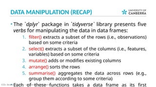
• In data wrangling, most likely, you need to perform series of
operations (i.e. verbs) on the same data.
• This will need you to create intermediate tables temporarily to
save the results to be processed with the next operations.
• R provides an elegant way to perform series of operations on
the same data in one go via using the pipe operator %>%
original data select filter
→ →
©Dr. Ibrahim Radwan – University of Canberra
16 %>% sqrt() %>% log2()
[1] 2
F(x) is the same as
x %>% F
THE PIPE OPERATOR %>% (2)
• In a previous `nycflights` example, there were three
steps to extract the relationship between the distance
and the delay of the flights per destination.
1. Group flights by destination.
2. Summarise to compute distance, average delay, and
number of flights.
3. Filter to remove noisy points
This can be achieved by using the pipe operator:
©Dr. Ibrahim Radwan – University of Canberra
delay <- df %>%
group_by(dest) %>%
summarise(count= n(), dist= mean(distance, na.rm =
TRUE), delay= mean(arr_delay, na.rm = TRUE)) %>%
filter(count > 20, dest != 'HNL')
TIDY DATA
• There are three interrelated rules which make a dataset tidy:
1. Each variable must have its own column.
2. Each observation must have its own row.
3. Each value must have its own cell.
©Dr. Ibrahim Radwan – University of Canberra
Credit: R for Data Science
Having our data in a tidy
format is a crucial step for
data manipulation and
exploring
TIDY DATA (2)
• Example of non-tidy data:
©Dr. Ibrahim Radwan – University of Canberra
The data are not tidy, why?
1. Each row includes several
observations and
2. One of the variables, year, is stored in
the header.
country 1960 1961 1962 1963 1964 1965
1
German
y 2.41 2.44 2.47 2.49 2.49 2.48
2
South
Korea 6.16 5.99 5.79 5.57 5.36 5.16
TIDY DATA (3)
©Dr. Ibrahim Radwan – University of Canberra
index country year fertility
1 Germany 1960 2.41
2
South
Korea 1960 6.16
3 Germany 1961 2.44
4
South
Korea 1961 5.99
5 Germany 1962 2.47
6
South
Korea 1962 5.79
To make the data in previous slide
tidy, we need to convert it from
wide to long. To do so, we first
define the variables embedded in
the data. Here we have 3
variables. Then we tabulate the
data within their corresponding
variables.
Now, this dataset is tidy because
each row presents one observation
with the three variables being
county, year and fertility rate.
TIDY DATA GRAMMAR
• The `tidyr` package presents four main verbs/functions
to tide up the data:
1. gather() collapses multiple columns into key-value
pairs. It produces a “long” data format from a “wide”
one.
2. spread() takes two columns (key & value), and spreads
into multiple columns: it makes “long” data wider. This
is the reverse of gather.
3. unite() unites multiple columns into one
4. separate() takes a column and divides it into multiple
columns
©Dr. Ibrahim Radwan – University of Canberra
GATHER DATA
©Dr. Ibrahim Radwan – University of Canberra
gather(data,key, value, …)
data: A data frame
key, value: Names of key and value columns to create in output
…: Specification of columns to gather. Allowed values are:
variable names
SPREAD DATA
©Dr. Ibrahim Radwan – University of Canberra
spread(data,key, value)
data: A data frame
key: The (unquoted) name of the column whose values will be used
as column headings.
value: The (unquoted) names of the column whose values will
populate the cells.
UNITE DATA
©Dr. Ibrahim Radwan – University of Canberra
unite(data, col, … , sep=)
The function unite() takes multiple columns and paste them
together into one-character column.
data: A data frame
col: The new (unquoted) name of column to add.
sep: Separator to use between values
SEPARATE DATA
©Dr. Ibrahim Radwan – University of Canberra
separate(data, col, into, sep=)
The sperate() function takes values inside a single character
column and separates them into multiple columns.
data: A data frame
col: Unquoted column names
into: Character vector specifying the names of new variables to be
created.
sep: Separator character between columns.
TIDY DATA (WRAP-UP)
• You should tidy your data for easier data analysis. The package tidyr provides the
following functions.
­ Collapse multiple columns together into key-value pairs (long data format):
 gather(data, key, value, …)
­ Spread key-value pairs into multiple columns (wide data format):
 spread(data, key, value)
­ Unite multiple columns into one:
 unite(data, col, …)
­ Separate one columns into multiple:
 separate(data, col, into)
©Dr. Ibrahim Radwan – University of Canberra
A CASE STUDY
• We have two files, which are downloaded from
“data.gov.au” about the unemployment rate per
gender for persons with disabilities between 1978 and
2017
• Can we inspect the unemployment rate over the
various age groups?
©Dr. Ibrahim Radwan – University of Canberra
We will do this task step-by-step in
R-studio and the code can
downloaded from Canvas
RECOMMENDED READING
• You are recommended to read chapters 12 from the
“R for Data Science” book:
­ https://r4ds.had.co.nz/tidy-data.html
©Dr. Ibrahim Radwan – University of Canberra
ANNOUNCEMENTS
• Next week is the semester break, no classes
• The week 9 online test is anticipated to be released
Monday of week 9
• ISEQ2 is open since yesterday for a week, let us hear
from you
©Dr. Ibrahim Radwan – University of Canberra

description description description description

  • 1.
    Lecture 7 Introduction toData Science (11372 & G 11516) Semester 1 2023 INTRODUCTION TO DATA SCIENCE Dr. Ibrahim Radwan
  • 2.
    OUTLINE • Data Wrangling(Recap) • Tidy data • A case study ©Dr. Ibrahim Radwan – University of Canberra
  • 3.
    DATA WRANGLING • Practically,we have three main components to wrangle the data ©Dr. Ibrahim Radwan – University of Canberra Imp ort Transform Visuali se tidyr dplyr ggplot 2 Tide Manipul ate read r
  • 4.
    DATA IMPORT (RECAP) ©Dr.Ibrahim Radwan – University of Canberra Comma Delimited Files read_csv("file.csv") Semi-colon Delimited Files read_csv2("file2.csv") Files with Any Delimiter read_delim("file.txt", delim = "|") Tab Delimited Files read_tsv("file.tsv") Also read_table() Comma delimited file write_csv(x, path, na = "NA", append = FALSE, col_names = !append) File with arbitrary delimiter write_delim(x, path, delim = " ", na = "NA", append = FALSE, col_names = !append) To save data into csv or txt file
  • 5.
    DATA MANIPULATION (RECAP) •The `dplyr` package in `tidyverse` library presents five verbs for manipulating the data in data frames: 1. filter() extracts a subset of the rows (i.e., observations) based on some criteria 2. select() extracts a subset of the columns (i.e., features, variables) based on some criteria 3. mutate() adds or modifies existing columns 4. arrange() sorts the rows 5. summarise() aggregates the data across rows (e.g., group them according to some criteria) • Each of these functions takes a data frame as its first ©Dr. Ibrahim Radwan – University of Canberra
  • 6.
    AGGREGATE (SUMMARISE) ©Dr. IbrahimRadwan – University of Canberra # call the required libraries library(tidyverse) library(nycflights13) df <- flights # extract a statistical metric from variable / variables of the data summarise(df, delay = mean(dep_delay, na.rm = TRUE)) summarise(dataframe, agg_func(col_name)) P L<=P n 1 summarise() is not terribly useful unless we pair it with group_by() Aggregation functions such as mean, sd, var, median, min and max There is also summarise_each(dataframe, funs(aggregation_func))
  • 7.
    AGGREGATE WITH GROUPING ©Dr.Ibrahim Radwan – University of Canberra # group the data of the flights by the date by_day <- group_by(flights, year, month, day) # get the average delay per date/day summarise(by_day, delay = mean(dep_delay, na.rm = TRUE)) # Imagine that we want to explore the relationship between the distance and average delay for each location. by_dest <- group_by(flights, dest) # extract the number of flights, average distance and average delay for each destination delay <- summarise(by_dest, count= n(), dist= mean(distance, na.rm = TRUE), delay= mean(arr_delay, na.rm = TRUE) ) # visualise to understand the relationship ggplot(data= delay, mapping=aes(x= dist, y= delay)) + geom_point(aes(size= count), alpha= 1/ 3) + geom_smooth() group_by(dataframe, col_name) P L<=P n 1
  • 8.
    PIPE OPERATOR %>% •In data wrangling, most likely, you need to perform series of operations (i.e. verbs) on the same data. • This will need you to create intermediate tables temporarily to save the results to be processed with the next operations. • R provides an elegant way to perform series of operations on the same data in one go via using the pipe operator %>% original data select filter → → ©Dr. Ibrahim Radwan – University of Canberra 16 %>% sqrt() %>% log2() [1] 2 F(x) is the same as x %>% F
  • 9.
    THE PIPE OPERATOR%>% (2) • In a previous `nycflights` example, there were three steps to extract the relationship between the distance and the delay of the flights per destination. 1. Group flights by destination. 2. Summarise to compute distance, average delay, and number of flights. 3. Filter to remove noisy points This can be achieved by using the pipe operator: ©Dr. Ibrahim Radwan – University of Canberra delay <- df %>% group_by(dest) %>% summarise(count= n(), dist= mean(distance, na.rm = TRUE), delay= mean(arr_delay, na.rm = TRUE)) %>% filter(count > 20, dest != 'HNL')
  • 10.
    TIDY DATA • Thereare three interrelated rules which make a dataset tidy: 1. Each variable must have its own column. 2. Each observation must have its own row. 3. Each value must have its own cell. ©Dr. Ibrahim Radwan – University of Canberra Credit: R for Data Science Having our data in a tidy format is a crucial step for data manipulation and exploring
  • 11.
    TIDY DATA (2) •Example of non-tidy data: ©Dr. Ibrahim Radwan – University of Canberra The data are not tidy, why? 1. Each row includes several observations and 2. One of the variables, year, is stored in the header. country 1960 1961 1962 1963 1964 1965 1 German y 2.41 2.44 2.47 2.49 2.49 2.48 2 South Korea 6.16 5.99 5.79 5.57 5.36 5.16
  • 12.
    TIDY DATA (3) ©Dr.Ibrahim Radwan – University of Canberra index country year fertility 1 Germany 1960 2.41 2 South Korea 1960 6.16 3 Germany 1961 2.44 4 South Korea 1961 5.99 5 Germany 1962 2.47 6 South Korea 1962 5.79 To make the data in previous slide tidy, we need to convert it from wide to long. To do so, we first define the variables embedded in the data. Here we have 3 variables. Then we tabulate the data within their corresponding variables. Now, this dataset is tidy because each row presents one observation with the three variables being county, year and fertility rate.
  • 13.
    TIDY DATA GRAMMAR •The `tidyr` package presents four main verbs/functions to tide up the data: 1. gather() collapses multiple columns into key-value pairs. It produces a “long” data format from a “wide” one. 2. spread() takes two columns (key & value), and spreads into multiple columns: it makes “long” data wider. This is the reverse of gather. 3. unite() unites multiple columns into one 4. separate() takes a column and divides it into multiple columns ©Dr. Ibrahim Radwan – University of Canberra
  • 14.
    GATHER DATA ©Dr. IbrahimRadwan – University of Canberra gather(data,key, value, …) data: A data frame key, value: Names of key and value columns to create in output …: Specification of columns to gather. Allowed values are: variable names
  • 15.
    SPREAD DATA ©Dr. IbrahimRadwan – University of Canberra spread(data,key, value) data: A data frame key: The (unquoted) name of the column whose values will be used as column headings. value: The (unquoted) names of the column whose values will populate the cells.
  • 16.
    UNITE DATA ©Dr. IbrahimRadwan – University of Canberra unite(data, col, … , sep=) The function unite() takes multiple columns and paste them together into one-character column. data: A data frame col: The new (unquoted) name of column to add. sep: Separator to use between values
  • 17.
    SEPARATE DATA ©Dr. IbrahimRadwan – University of Canberra separate(data, col, into, sep=) The sperate() function takes values inside a single character column and separates them into multiple columns. data: A data frame col: Unquoted column names into: Character vector specifying the names of new variables to be created. sep: Separator character between columns.
  • 18.
    TIDY DATA (WRAP-UP) •You should tidy your data for easier data analysis. The package tidyr provides the following functions. ­ Collapse multiple columns together into key-value pairs (long data format):  gather(data, key, value, …) ­ Spread key-value pairs into multiple columns (wide data format):  spread(data, key, value) ­ Unite multiple columns into one:  unite(data, col, …) ­ Separate one columns into multiple:  separate(data, col, into) ©Dr. Ibrahim Radwan – University of Canberra
  • 19.
    A CASE STUDY •We have two files, which are downloaded from “data.gov.au” about the unemployment rate per gender for persons with disabilities between 1978 and 2017 • Can we inspect the unemployment rate over the various age groups? ©Dr. Ibrahim Radwan – University of Canberra We will do this task step-by-step in R-studio and the code can downloaded from Canvas
  • 20.
    RECOMMENDED READING • Youare recommended to read chapters 12 from the “R for Data Science” book: ­ https://r4ds.had.co.nz/tidy-data.html ©Dr. Ibrahim Radwan – University of Canberra
  • 21.
    ANNOUNCEMENTS • Next weekis the semester break, no classes • The week 9 online test is anticipated to be released Monday of week 9 • ISEQ2 is open since yesterday for a week, let us hear from you ©Dr. Ibrahim Radwan – University of Canberra