Data Assimilation in Numerical Weather Prediction Models

Data Assimilation in Numerical Weather Prediction models
África Periáñez
DWD, Germany
CERN, Geneva, February 20, 2014

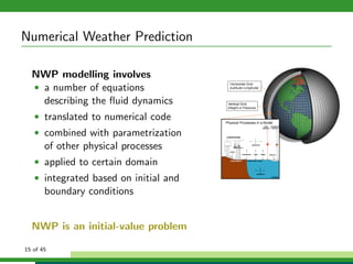
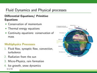
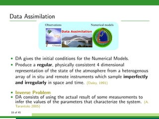
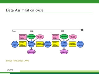
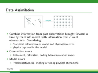
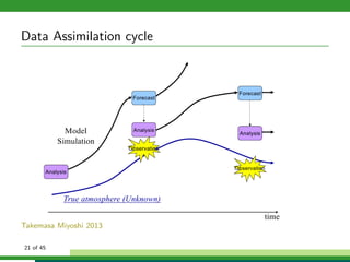
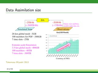
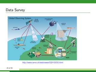
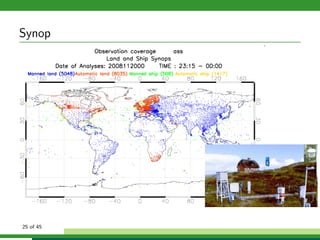
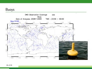
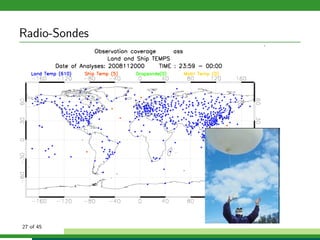
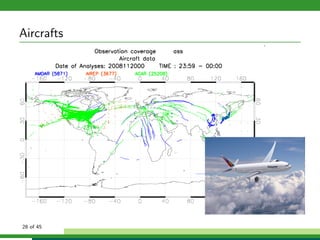
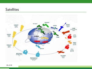
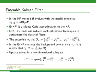
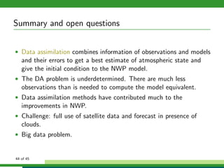
Outline
Numerical Weather Prediction
Can Numerics Help?
Introduction to Numerical Weather Prediction models
Dynamical Systems, Inverse Problems and Data Assimilation
Fluid Dynamics and Physical Processes
Data Assimilation
Measurements: Stations, Sondes, Planes, Satellites
Data Assimilation in DWD
Basic Approach
Ensemble Kalman Filter
Conclusions
2 of 45

Outline
Can Numerics Help?
Data Assimilation
Basic Approach
Conclusions
3 of 45

Weather is Relevant
Warn and Protect
Plan Travel
4 of 45

Weather is Relevant
Logistics
Rivers and Environment
Air Control
5 of 45

Outline
Can Numerics Help?
Data Assimilation
Basic Approach
Conclusions
6 of 45

Deﬁnitions
• NWP processes current weather observations
through computer models to forecast the future
state of weather.
• Data Assimilation computes the initial conditions
for the NWP model.
◦ the data available (105) is not enough to
initialize current models with 107 degrees of
freedom
◦ need spatial and time interpolation
◦ sometimes variables are not measured directly
◦ we do not know the truth
• Our system is: ’a 3d grid of the atmosphere, with
current data, and equations that describe
atmosphere dynamics.’
7 of 45

Remarks on the History of Weather Prediction I
• In 1901 Cleveland Abbe founded the United States Weather
Bureau. He suggested that the atmosphere followed the
principles of thermodynamics and hydrodynamics
• In 1904, Vilhelm Bjerknes proposed a two-step procedure for
model-based weather forecasting. First, an analysis step of
data assimilation to generate initial conditions, then a
forecasting step solving the initial value problem.
• In 1922, Lewis Fry Richardson carried out the first attempt to
perform the weather forecast numerically.
• In 1950, a team of the American meteorologists Jule Charney,
Philip Thompson, Larry Gates, and Norwegian meteorologist
Ragnar Fjörtoft and the applied mathematician John von
Neumann, succeeded in the first numerical weather forecast
using the ENIAC digital computer.
Bjerknes
8 of 45

Remarks on the History of Weather Prediction II
1962
Nimbus 1: 1964
• In September 1954, Carl-Gustav Rossby’s group at the Swedish
Meteorological and Hydrological Institute produced the ﬁrst
operational forecast (i.e. routine predictions for practical use)
based on the barotropic equation. Operational numerical weather
prediction in the United States began in 1955 under the Joint
Numerical Weather Prediction Unit (JNWPU), a joint project by
the U.S. Air Force, Navy, and Weather Bureau.
• In 1959, Karl-Heinz Hinkelmann produced the ﬁrst reasonable
primitive equation forecast, 37 years after Richardson’s failed
attempt. Hinkelmann did so by removing high-frequency noise
from the numerical model during initialization.
• In 1966, West Germany and the United States began producing
operational forecasts based on primitive-equation models, followed
by the United Kingdom in 1972, and Australia in 1977.
9 of 45

Operational Centers
Met Oﬃce
11 of 45

Comparison Northern and Southern hemispheres
12 of 45

Outline
Can Numerics Help?
Data Assimilation
Basic Approach
Conclusions
13 of 45

Outline
Can Numerics Help?
Data Assimilation
Basic Approach
Conclusions
14 of 45

NWP modelling involves
• a number of equations
describing the ﬂuid dynamics
• translated to numerical code
• combined with parametrization
of other physical processes
• applied to certain domain
• integrated based on initial and
boundary conditions
NWP is an initial-value problem
15 of 45

Fluid Dynamics and Physical processes
Differential Equations/ Primitive
Equations
• Conservation of momentum
• Thermal energy equations
• Continuity equations: conservation of
mass
Multiphysics Processes
1. Fluid flow, synoptic flow, convection,
turbulence
2. Radiation from the sun
3. Micro-Physics, rain formation
4. Ice growth, snow dynamics
16 of 45

Outline
Can Numerics Help?
Data Assimilation
Basic Approach
Conclusions
17 of 45

Data Assimilation
• DA gives the initial conditions for the Numerical Models.
• Produce a regular, physically consistent 4 dimensional
representation of the state of the atmosphere from a heterogenous
array of in situ and remote instruments which sample imperfectly
and irregularly in space and time. (Daley, 1991)
• Inverse Problem
• DA consists of using the actual result of some measurements to
infer the values of the parameters that characterize the system. (A.
Tarantolo 2005)
18 of 45

Data Assimilation cycle
Soroja Polavarapu 2008
19 of 45

Data Assimilation
• Combine information from past observations brought forward in
time by the NWP model, with information from current
observations. Considering:
◦ Statistical information on model and observation error.
◦ physics captured in the model
• Observation errors
◦ Instrument, calibration, coding telecomunication errors
• Model errors
◦ ’representativeness’, missing or wrong physical phenomena
20 of 45

Data Assimilation cycle
Takemasa Miyoshi 2013
21 of 45

Data Assimilation size
Takemasa Miyoshi 2013
22 of 45

Outline
Can Numerics Help?
Data Assimilation
Basic Approach
Conclusions
23 of 45

Outline
Can Numerics Help?
Data Assimilation
Basic Approach
Conclusions
34 of 45

DA in DWD
• Research and Development
• Section on Modelling:
◦ Unit Num. Modelling
◦ Unit Data Assimilation
◦ Unit Physics
◦ Unit Veriﬁcation
35 of 45

Modelling of the Atmosphere: Geometry
• GME/ICON
Resolution 30km
• COSMO-EU
Resolution 7km
• COSMO-DE
Resolution 2.8km
36 of 45

Model and Assimilation Systems at DWD
• Current:
◦ GME 30Km 3DVar
◦ COSMO-EU 7Km Nudging
◦ COSMO-DE 2.8Km Nudging
• Next Future (2014):
◦ ICON Global, Regional grid reﬁnement,
non-hydrostatic, deterministic: 13Km EPS:20Km
Hybrid 3DVar-LETKF
◦ COSMO-DE both deterministic and EPS: 2km
LETKF
37 of 45

Outline
Can Numerics Help?
Data Assimilation
Basic Approach
Conclusions
38 of 45

Basic Approach
Let H be the observation operator mapping the state ϕ onto the
measurements f . Then we need to ﬁnd ϕ by solving the equation
H(ϕ) = f ,
where H−1 is not lineal. When we have some initial guess ϕ(b), we
transform the equation into
H(ϕ − ϕ(b)
) = f − Hϕ(b)
,
with the incremental form
ϕ = ϕ(b)
+ H−1
(f − Hϕ(b)
).
39 of 45

Least Squares
In order to find out ϕ we should minimize the functional
J(ϕ) := ϕ − ϕ(b) 2
+ f − Hϕ(b) 2
.
The normal equations are obtained from first order optimality
conditions
ϕJ = 0.
Usually, the relation between variables at different points is
incorporated by using covariances/weighted norms:
J(ϕ) := ϕ − ϕ(b) 2
B−1 + f − Hϕ(b) 2
R−1 ,
The update formula is now
ϕ(a)
= ϕ(b)
+ BH∗
(R + HBH∗
)−1
(f − Hϕ(b)
)
40 of 45

Outline
Can Numerics Help?
Data Assimilation
Basic Approach
Conclusions
41 of 45

• In the KF method B evolves with the model dynamics:
Bk+1 = MBkM∗.
• EnKF1 is a Monte Carlo approximation to the KF.
• EnKF methods use reduced rank estimation techniques to
aproximate the classical ﬁlters.
• The ensemble matrix Qk := ϕ
(1)
k − ϕ
(b)
k , ..., ϕ
(L)
k − ϕ
(b)
k .
• In the EnKF methods the background convariance matrix is
represented by B := 1
L−1QkQ∗
k .
• Update solved in a low-dimensional subspace
U(L)
:= span{ϕ
(1)
k − ϕ
(b)
k , ..., ϕ
(L)
k − ϕ
(b)
k }.
1
Evensen 199442 of 45

Outline
Can Numerics Help?
Data Assimilation
Basic Approach
Conclusions
43 of 45

Summary and open questions
• Data assimilation combines information of observations and models
and their errors to get a best estimate of atmospheric state and
give the initial condition to the NWP model.
• The DA problem is underdetermined. There are much less
observations than is needed to compute the model equivalent.
• Data assimilation methods have contributed much to the
improvements in NWP.
• Challenge: full use of satellite data and forecast in presence of
clouds.
• Big data problem.
44 of 45

Thank you for your attention!
• africa.perianez@dwd.de
• Data Assimilation Unit
45 of 45

Data Assimilation in Numerical Weather Prediction Models

Recommended

Recommended

More Related Content

What's hot

What's hot (20)

Similar to Data Assimilation in Numerical Weather Prediction Models

Similar to Data Assimilation in Numerical Weather Prediction Models (20)

Recently uploaded

Recently uploaded (20)

Data Assimilation in Numerical Weather Prediction Models