Downloaded 676 times


![© 2016 Continuum Analytics - Confidential & Proprietary
Without NumPyfrom math import sin, pi
def sinc(x):
if x == 0:
return 1.0
else:
pix = pi*x
return sin(pix)/pix
def step(x):
if x > 0:
return 1.0
elif x < 0:
return 0.0
else:
return 0.5
functions.py
>>> import functions as f
>>> xval = [x/3.0 for x in
range(-10,10)]
>>> yval1 = [f.sinc(x) for x
in xval]
>>> yval2 = [f.step(x) for x
in xval]
Python is a great language but
needed a way to operate quickly
and cleanly over multi-
dimensional arrays.](https://image.slidesharecdn.com/tdwiaccelerate-170405043601/85/Python-for-Data-Science-with-Anaconda-20-320.jpg)
![© 2016 Continuum Analytics - Confidential & Proprietary
With NumPy
from numpy import sin, pi
from numpy import vectorize
import functions as f
vsinc = vectorize(f.sinc)
def sinc(x):
pix = pi*x
val = sin(pix)/pix
val[x==0] = 1.0
return val
vstep = vectorize(f.step)
def step(x):
y = x*0.0
y[x>0] = 1
y[x==0] = 0.5
return y
>>> import functions2 as f
>>> from numpy import *
>>> x = r_[-10:10]/3.0
>>> y1 = f.sinc(x)
>>> y2 = f.step(x)
functions2.py
Offers N-D array, element-by-element
functions, and basic random numbers,
linear algebra, and FFT capability for
Python
http://numpy.org
Fiscally sponsored by NumFOCUS](https://image.slidesharecdn.com/tdwiaccelerate-170405043601/85/Python-for-Data-Science-with-Anaconda-21-320.jpg)


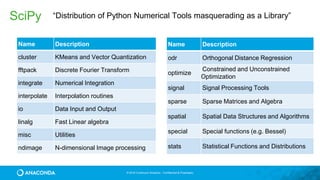
![© 2016 Continuum Analytics - Confidential & Proprietary
NumPy Examples
2d array
3d array
[439 472 477]
[217 205 261 222 245 238]
9.98330639789 2.96677717122](https://image.slidesharecdn.com/tdwiaccelerate-170405043601/85/Python-for-Data-Science-with-Anaconda-24-320.jpg)
![© 2016 Continuum Analytics - Confidential & Proprietary
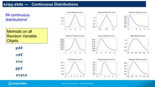
NumPy Slicing (Selection)
>>> a[0,3:5]
array([3, 4])
>>> a[4:,4:]
array([[44, 45],
[54, 55]])
>>> a[:,2]
array([2,12,22,32,42,52])
>>> a[2::2,::2]
array([[20, 22, 24],
[40, 42, 44]])](https://image.slidesharecdn.com/tdwiaccelerate-170405043601/85/Python-for-Data-Science-with-Anaconda-25-320.jpg)


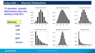

![© 2016 Continuum Analytics - Confidential & Proprietary
a powerful plotting engine
import matplotlib.pyplot as plt
import scipy.misc as misc
im = misc.face()
ax = plt.imshow(im)
plt.title('Racoon Face of size
%d x %d' % im.shape[:2])
plt.savefig(‘face.png’)](https://image.slidesharecdn.com/tdwiaccelerate-170405043601/85/Python-for-Data-Science-with-Anaconda-35-320.jpg)
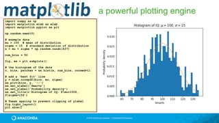
![© 2016 Continuum Analytics - Confidential & Proprietary
a powerful plotting engine
import matplotlib.pyplot as plt
import numpy as np
with plt.xkcd():
fig = plt.figure()
ax = fig.add_axes((0.1, 0.2, 0.8, 0.7))
ax.spines['right'].set_color('none')
ax.spines['top'].set_color('none')
plt.xticks([])
plt.yticks([])
ax.set_ylim([-30, 10])
data = np.ones(100)
data[70:] -= np.arange(30)
plt.annotate('THE DAY I REALIZEDnI COULD
COOK BACONnWHENEVER I WANTED’,
xy=(70, 1),
arrowprops=dict(arrowstyle=‘->'),
xytext=(15, -10))
plt.plot(data)
plt.xlabel('time')
plt.ylabel('my overall health')
fig.text(0.5, 0.05, '"Stove Ownership" from
xkcd by Randall Monroe',
ha='center')](https://image.slidesharecdn.com/tdwiaccelerate-170405043601/85/Python-for-Data-Science-with-Anaconda-36-320.jpg)


![© 2016 Continuum Analytics - Confidential & Proprietary
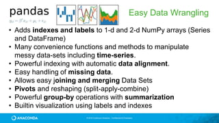
Easy Data Wrangling
medals = pd.read_csv('data/medals.csv', index_col='name')
medals.head()
gold = medals['medal'] == 'gold'
won = medals['count'] > 0
medals.loc[gold & won, 'count'].sort_values().plot(kind='bar', figsize=(12,8))](https://image.slidesharecdn.com/tdwiaccelerate-170405043601/85/Python-for-Data-Science-with-Anaconda-41-320.jpg)
![© 2016 Continuum Analytics - Confidential & Proprietary
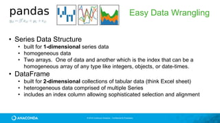
Easy Data Wrangling
df = pd.read_excel("data/pbpython/salesfunnel.xlsx")
df.head()
table = pd.pivot_table(df,
index=["Manager","Rep","Product"],
values=["Price","Quantity"],
aggfunc=[np.sum,np.mean])](https://image.slidesharecdn.com/tdwiaccelerate-170405043601/85/Python-for-Data-Science-with-Anaconda-43-320.jpg)


![© 2016 Continuum Analytics - Confidential & Proprietary
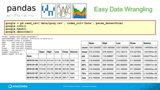
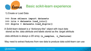
Basic scikit-learn experience
3) Train the Model
>>> clf.fit(data[:-1], labels[:-1])
Models have a “fit” method which updates the parameters-to-be-estimated in
the model in-place so that after fitting the model is “trained”
For validation and scoring you need to leave out some of the data to use
later. cross-validation (e.g. k-fold) techniques can also be parallelized easily.
Here we “leave-one-out” (or n-fold)](https://image.slidesharecdn.com/tdwiaccelerate-170405043601/85/Python-for-Data-Science-with-Anaconda-49-320.jpg)
![© 2016 Continuum Analytics - Confidential & Proprietary
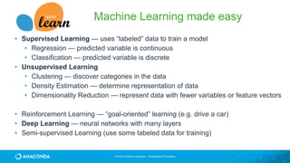
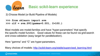
Basic scikit-learn experience
4) Predict new values
>>> clf.predict(data[-1:])
Prediction of new data uses the trained parameters of the model. Cross-
validation can be used to understand how sensitive the model is to different
partitions of the data.
>>> from sklearn.model_selection import cross_val_score
>>> scores = cross_val_score(clf, data, target, cv=10)
array([ 0.96…, 1. …, 0.96… , 1. ])](https://image.slidesharecdn.com/tdwiaccelerate-170405043601/85/Python-for-Data-Science-with-Anaconda-50-320.jpg)

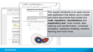


![© 2016 Continuum Analytics - Confidential & Proprietary
tiles = gv.WMTS(WMTSTileSource(url='https://server.arcgisonline.com/ArcGIS/rest/services/'
'World_Imagery/MapServer/tile/{Z}/{Y}/{X}.jpg'))
tile_options = dict(width=800,height=475,xaxis=None,yaxis=None,bgcolor='black',show_grid=False)
passenger_counts = sorted(df.passenger_count.unique().tolist())
class Options(hv.streams.Stream):
alpha = param.Magnitude(default=0.75, doc="Alpha value for the map opacity")
colormap = param.ObjectSelector(default=cm["fire"], objects=cm.values())
plot = param.ObjectSelector(default="pickup", objects=["pickup","dropoff"])
passengers = param.ObjectSelector(default=1, objects=passenger_counts)
def make_plot(self, x_range=None, y_range=None, **kwargs):
map_tiles = tiles(style=dict(alpha=self.alpha), plot=tile_options)
df_filt = df[df.passenger_count==self.passengers]
points = hv.Points(gv.Dataset(df_filt, kdims=[self.plot+'_x', self.plot+'_y'], vdims=[]))
taxi_trips = datashade(points, width=800, height=475, x_sampling=1, y_sampling=1,
cmap=self.colormap, element_type=gv.Image,
dynamic=False, x_range=x_range, y_range=y_range)
return map_tiles * taxi_trips
selector = Options(name="")
paramnb.Widgets(selector, callback=selector.update)
hv.DynamicMap(selector.make_plot, kdims=[], streams=[selector, RangeXY()])
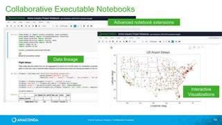
Data Widgets and
Applications from
Jupyter Notebooks!
https://anaconda.org/jbednar/nyc_taxi-paramnb/notebook](https://image.slidesharecdn.com/tdwiaccelerate-170405043601/85/Python-for-Data-Science-with-Anaconda-63-320.jpg)


![© 2016 Continuum Analytics - Confidential & Proprietary
Image Processing
@jit('void(f8[:,:],f8[:,:],f8[:,:])')
def filter(image, filt, output):
M, N = image.shape
m, n = filt.shape
for i in range(m//2, M-m//2):
for j in range(n//2, N-n//2):
result = 0.0
for k in range(m):
for l in range(n):
result += image[i+k-m//2,j+l-n//2]*filt[k, l]
output[i,j] = result
~1500x speed-up](https://image.slidesharecdn.com/tdwiaccelerate-170405043601/85/Python-for-Data-Science-with-Anaconda-69-320.jpg)


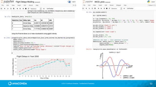
![© 2016 Continuum Analytics - Confidential & Proprietary
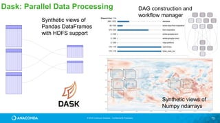
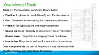
Dask
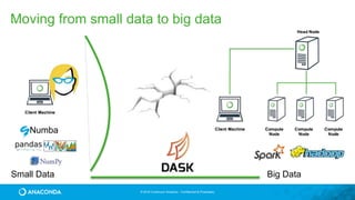
• Started as part of Blaze in early 2014.
• General parallel programming engine
• Flexible and therefore highly suited for
• Commodity Clusters
• Advanced Algorithms
• Wide community adoption and use
conda install -c conda-forge dask
pip install dask[complete] distributed --upgrade](https://image.slidesharecdn.com/tdwiaccelerate-170405043601/85/Python-for-Data-Science-with-Anaconda-72-320.jpg)

![© 2016 Continuum Analytics - Confidential & Proprietary
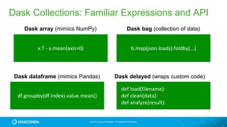
>>> import pandas as pd
>>> df = pd.read_csv('iris.csv')
>>> df.head()
sepal_length sepal_width petal_length petal_width species
0 5.1 3.5 1.4 0.2 Iris-setosa
1 4.9 3.0 1.4 0.2 Iris-setosa
2 4.7 3.2 1.3 0.2 Iris-setosa
3 4.6 3.1 1.5 0.2 Iris-setosa
4 5.0 3.6 1.4 0.2 Iris-setosa
>>> max_sepal_length_setosa = df[df.species
== 'setosa'].sepal_length.max()
5.7999999999999998
>>> import dask.dataframe as dd
>>> ddf = dd.read_csv('*.csv')
>>> ddf.head()
sepal_length sepal_width petal_length petal_width species
0 5.1 3.5 1.4 0.2 Iris-setosa
1 4.9 3.0 1.4 0.2 Iris-setosa
2 4.7 3.2 1.3 0.2 Iris-setosa
3 4.6 3.1 1.5 0.2 Iris-setosa
4 5.0 3.6 1.4 0.2 Iris-setosa
…
>>> d_max_sepal_length_setosa = ddf[ddf.species
== 'setosa'].sepal_length.max()
>>> d_max_sepal_length_setosa.compute()
5.7999999999999998
Dask Dataframes](https://image.slidesharecdn.com/tdwiaccelerate-170405043601/85/Python-for-Data-Science-with-Anaconda-78-320.jpg)


![© 2016 Continuum Analytics - Confidential & Proprietary
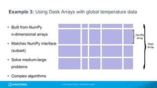
>>> import numpy as np
>>> np_ones = np.ones((5000, 1000))
>>> np_ones
array([[ 1., 1., 1., ..., 1., 1., 1.],
[ 1., 1., 1., ..., 1., 1., 1.],
[ 1., 1., 1., ..., 1., 1., 1.],
...,
[ 1., 1., 1., ..., 1., 1., 1.],
[ 1., 1., 1., ..., 1., 1., 1.],
[ 1., 1., 1., ..., 1., 1., 1.]])
>>> np_y = np.log(np_ones + 1)[:5].sum(axis=1)
>>> np_y
array([ 693.14718056, 693.14718056,
693.14718056, 693.14718056, 693.14718056])
>>> import dask.array as da
>>> da_ones = da.ones((5000000, 1000000),
chunks=(1000, 1000))
>>> da_ones.compute()
array([[ 1., 1., 1., ..., 1., 1., 1.],
[ 1., 1., 1., ..., 1., 1., 1.],
[ 1., 1., 1., ..., 1., 1., 1.],
...,
[ 1., 1., 1., ..., 1., 1., 1.],
[ 1., 1., 1., ..., 1., 1., 1.],
[ 1., 1., 1., ..., 1., 1., 1.]])
>>> da_y = da.log(da_ones + 1)[:5].sum(axis=1)
>>> np_da_y = np.array(da_y) #fits in memory
array([ 693.14718056, 693.14718056,
693.14718056, 693.14718056, …, 693.14718056])
# If result doesn’t fit in memory
>>> da_y.to_hdf5('myfile.hdf5', 'result')
Dask Arrays](https://image.slidesharecdn.com/tdwiaccelerate-170405043601/85/Python-for-Data-Science-with-Anaconda-81-320.jpg)


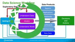

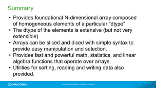
This document provides an overview of Continuum Analytics and Python for data science. It discusses how Continuum created two organizations, Anaconda and NumFOCUS, to support open source Python data science software. It then describes Continuum's Anaconda distribution, which brings together 200+ open source packages like NumPy, SciPy, Pandas, Scikit-learn, and Jupyter that are used for data science workflows involving data loading, analysis, modeling, and visualization. The document outlines how Continuum helps accelerate adoption of data science through Anaconda and provides examples of industries using Python for data science.