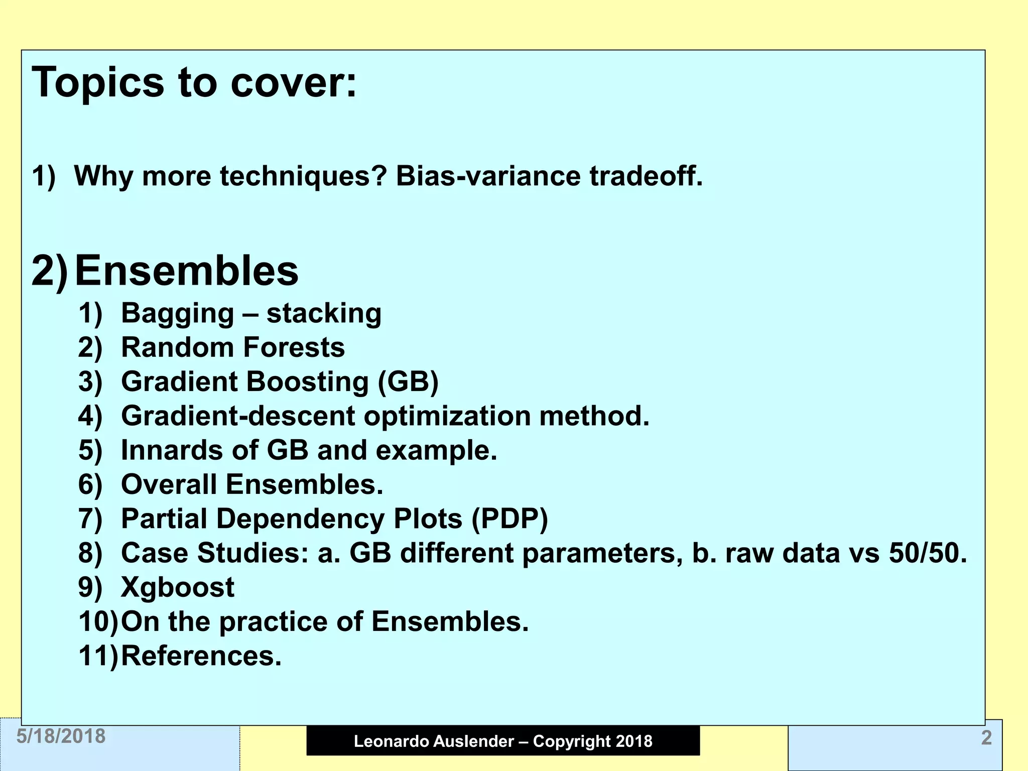
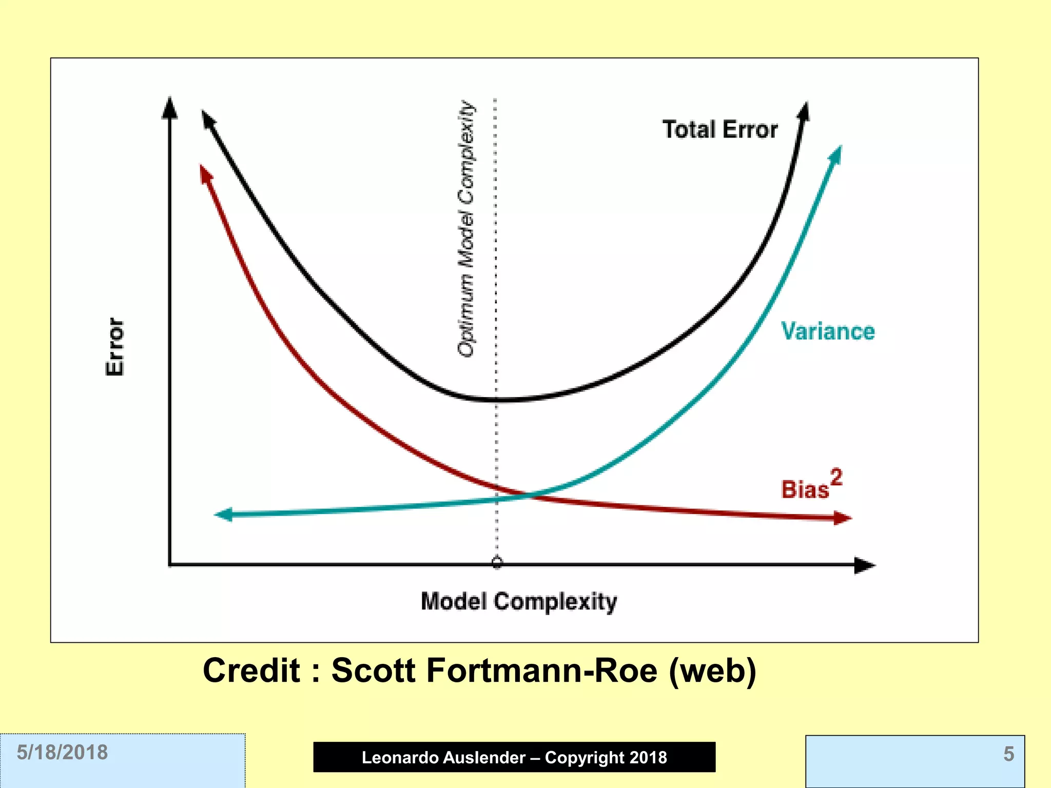
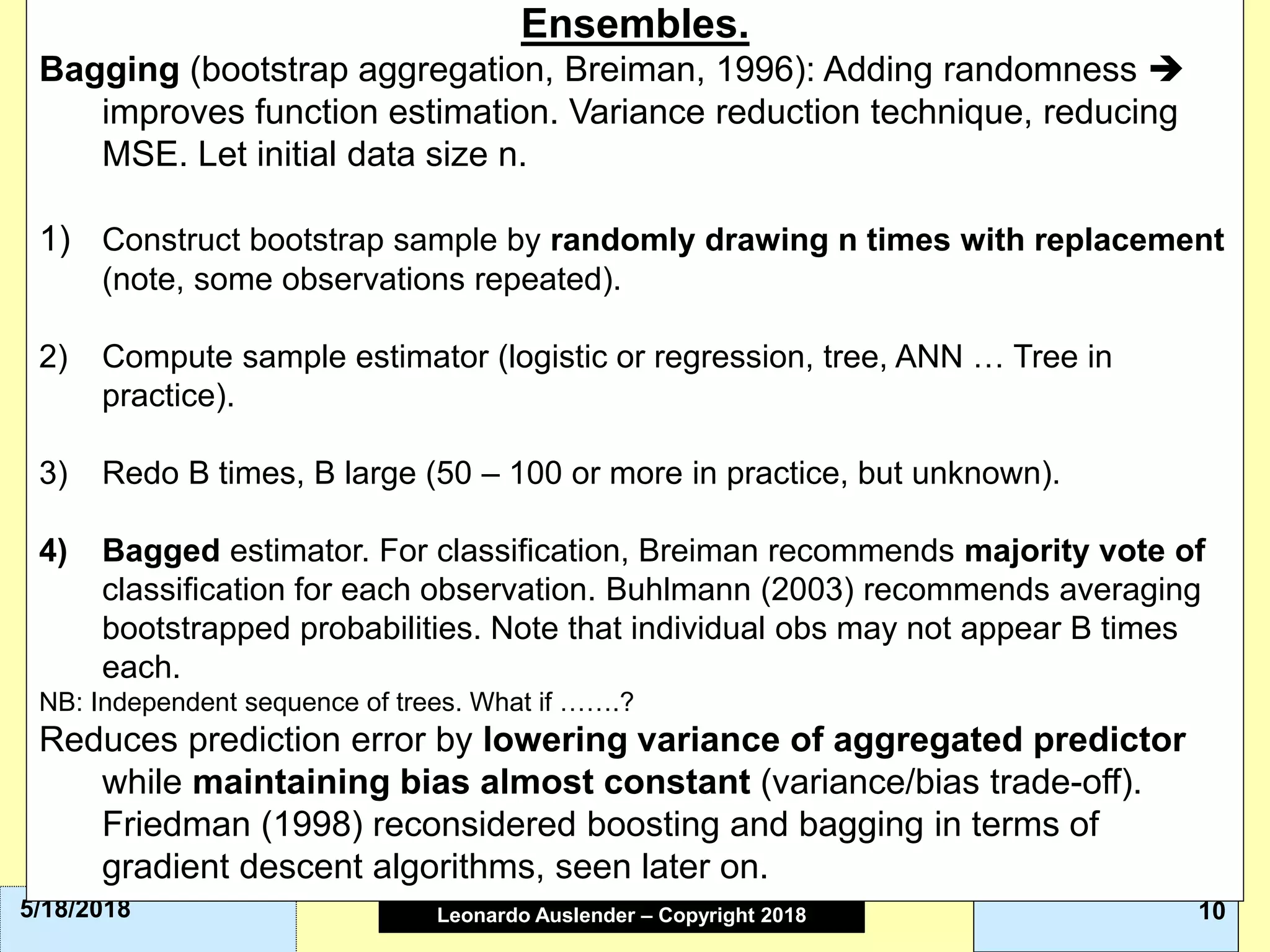
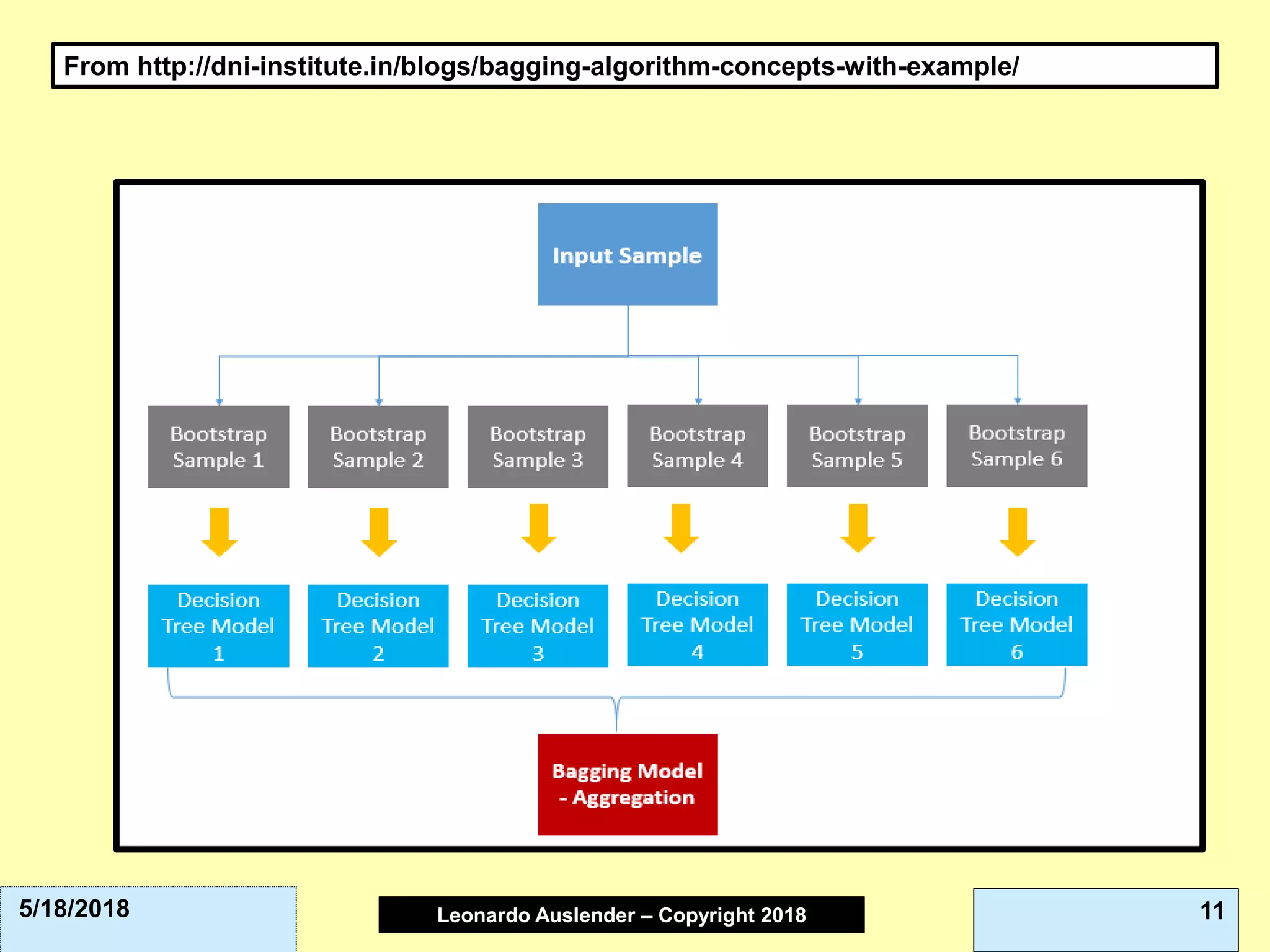
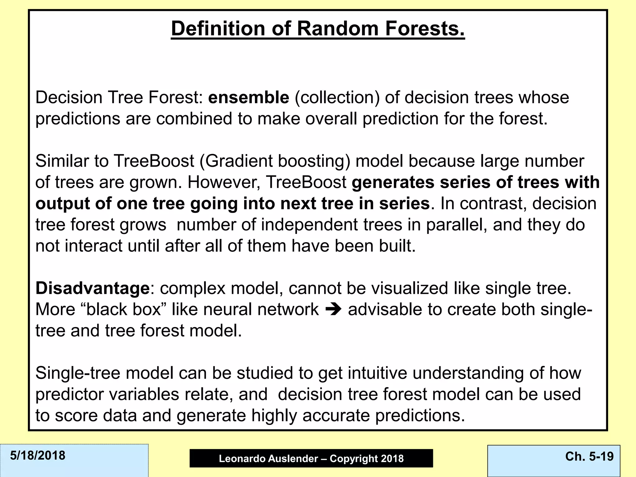
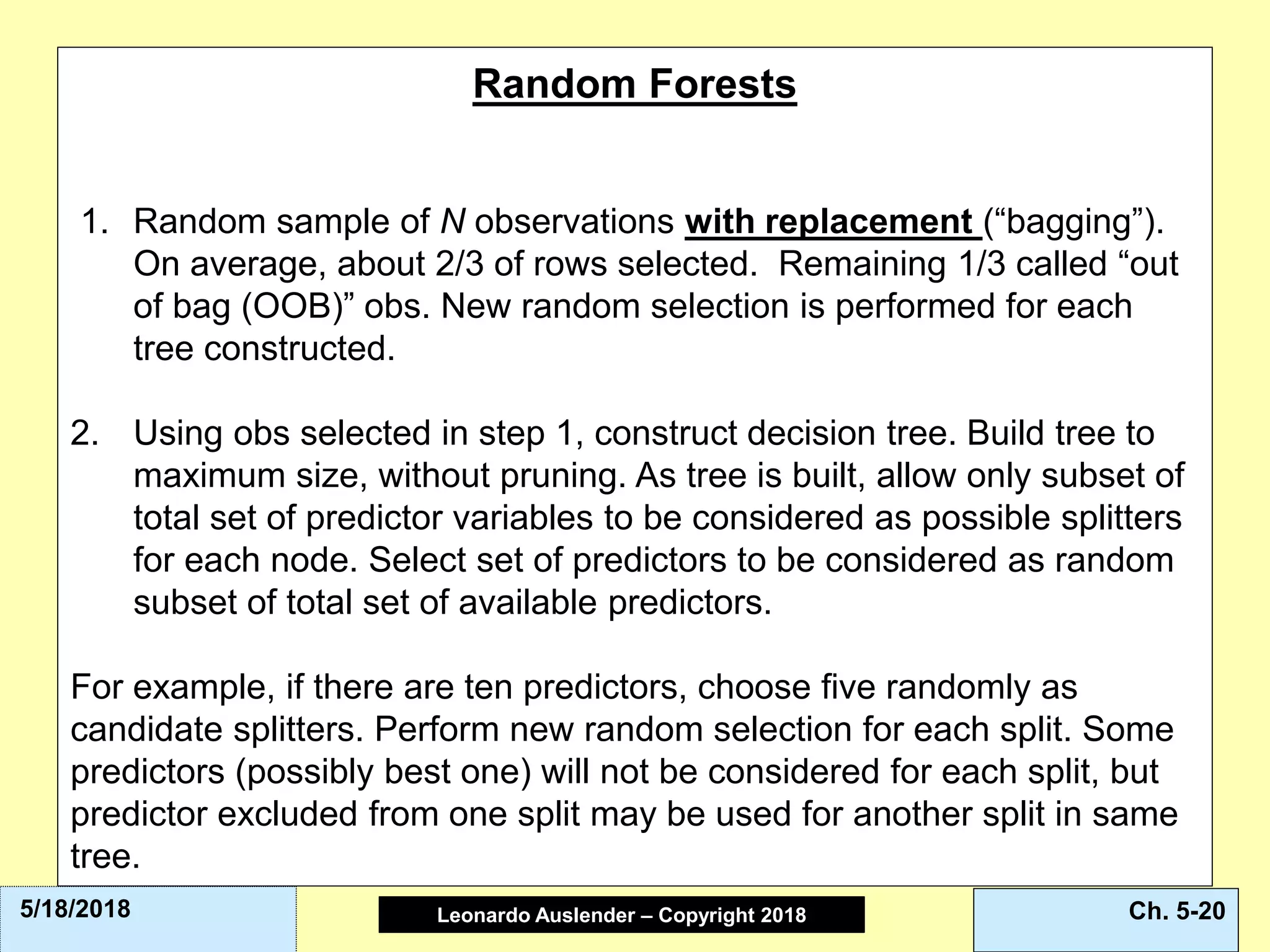
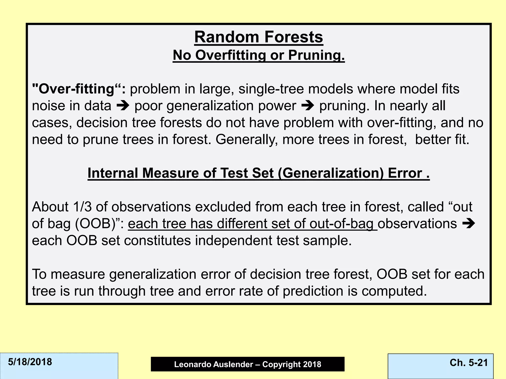
This document discusses ensemble methods and gradient boosting. It covers topics such as the bias-variance tradeoff, bagging, stacking, random forests, gradient boosting, and XGBoost. For random forests, it explains how they work by growing many decision trees on randomly sampled data and combining their predictions. It also discusses how random forests avoid overfitting and use out-of-bag samples to estimate generalization error.
Overview of tree algorithms from decision tree to xgboostTakami Sato
For my understanding, I surveyed popular tree algorithms on Machine Learning and their evolution. This is the first time I wrote a presentation in English. So, I am happy if you give me a feedback.
Overview of tree algorithms from decision tree to xgboostTakami Sato
For my understanding, I surveyed popular tree algorithms on Machine Learning and their evolution. This is the first time I wrote a presentation in English. So, I am happy if you give me a feedback.
Machine learning session6(decision trees random forrest)Abhimanyu Dwivedi
Concepts include decision tree with its examples. Measures used for splitting in decision tree like gini index, entropy, information gain, pros and cons, validation. Basics of random forests with its example and uses.
Automatic Differentiation and SciML in Reality: What can go wrong, and what t...Chris Rackauckas
How does automatic differentiation work, what happens when you apply it to equation solvers, and how can it go wrong? This talk is all about the details of how scientific machine learning (SciML) works. It goes into detail as to how neural networks are trained in the context of equation solvers, along with the numerical issues that can arise in the differentiation processes.
https://sciml.ai/
GDC2019 - SEED - Towards Deep Generative Models in Game DevelopmentElectronic Arts / DICE
Deep learning is becoming ubiquitous in Machine Learning (ML) research, and it's also finding its place in industry-related applications. Specifically, deep generative models have proven incredibly useful at generating and remixing realistic content from scratch, making themselves a very appealing technology in the field of AI-enhanced content authoring. As part of this year's Machine Learning Tutorial at the Game Developers Conference 2019 (GDC), Jorge Del Val from SEED will cover in an accessible manner the fundamentals of deep generative modeling, including some common algorithms and architectures. He will also discuss applications to game development and explore some recent advances in the field.
The attendee will gain basic understanding of the fundamentals of generative models and how to implement them. Also, attendees will grasp potential applications in the field of game development to inspire their work and companies. This talk does not require a mathematical or machine learning background, although previous knowledge on either of those is beneficial.
An Experimental Study about Simple Decision Trees for Bagging Ensemble on Dat...NTNU
Decision trees are simple structures used in supervised classification learning. The results of the application of decision trees in classification can be notably improved using ensemble methods such as Bagging, Boosting or Randomization, largely used in the literature. Bagging outperforms Boosting and Randomization in situations with classification noise. In this paper, we present an experimental study of the use of different simple decision tree methods for bagging ensemble in supervised classification, proving that simple credal decision trees (based on imprecise probabilities and uncertainty measures) outperforms the use of classical decision tree methods for this type of procedure when they are applied on datasets with classification noise.
Decision Trees for Classification: A Machine Learning AlgorithmPalin analytics
Decision Trees in Machine Learning - Decision tree method is a commonly used data mining method for establishing classification systems based on several covariates or for developing prediction algorithms for a target variable.
Similar to 4 2 ensemble models and grad boost part 1 (20)
Levelwise PageRank with Loop-Based Dead End Handling Strategy : SHORT REPORT ...Subhajit Sahu
Abstract — Levelwise PageRank is an alternative method of PageRank computation which decomposes the input graph into a directed acyclic block-graph of strongly connected components, and processes them in topological order, one level at a time. This enables calculation for ranks in a distributed fashion without per-iteration communication, unlike the standard method where all vertices are processed in each iteration. It however comes with a precondition of the absence of dead ends in the input graph. Here, the native non-distributed performance of Levelwise PageRank was compared against Monolithic PageRank on a CPU as well as a GPU. To ensure a fair comparison, Monolithic PageRank was also performed on a graph where vertices were split by components. Results indicate that Levelwise PageRank is about as fast as Monolithic PageRank on the CPU, but quite a bit slower on the GPU. Slowdown on the GPU is likely caused by a large submission of small workloads, and expected to be non-issue when the computation is performed on massive graphs.
Chatty Kathy - UNC Bootcamp Final Project Presentation - Final Version - 5.23...John Andrews
SlideShare Description for "Chatty Kathy - UNC Bootcamp Final Project Presentation"
Title: Chatty Kathy: Enhancing Physical Activity Among Older Adults
Description:
Discover how Chatty Kathy, an innovative project developed at the UNC Bootcamp, aims to tackle the challenge of low physical activity among older adults. Our AI-driven solution uses peer interaction to boost and sustain exercise levels, significantly improving health outcomes. This presentation covers our problem statement, the rationale behind Chatty Kathy, synthetic data and persona creation, model performance metrics, a visual demonstration of the project, and potential future developments. Join us for an insightful Q&A session to explore the potential of this groundbreaking project.
Project Team: Jay Requarth, Jana Avery, John Andrews, Dr. Dick Davis II, Nee Buntoum, Nam Yeongjin & Mat Nicholas
Opendatabay - Open Data Marketplace.pptxOpendatabay
Opendatabay.com unlocks the power of data for everyone. Open Data Marketplace fosters a collaborative hub for data enthusiasts to explore, share, and contribute to a vast collection of datasets.
First ever open hub for data enthusiasts to collaborate and innovate. A platform to explore, share, and contribute to a vast collection of datasets. Through robust quality control and innovative technologies like blockchain verification, opendatabay ensures the authenticity and reliability of datasets, empowering users to make data-driven decisions with confidence. Leverage cutting-edge AI technologies to enhance the data exploration, analysis, and discovery experience.
From intelligent search and recommendations to automated data productisation and quotation, Opendatabay AI-driven features streamline the data workflow. Finding the data you need shouldn't be a complex. Opendatabay simplifies the data acquisition process with an intuitive interface and robust search tools. Effortlessly explore, discover, and access the data you need, allowing you to focus on extracting valuable insights. Opendatabay breaks new ground with a dedicated, AI-generated, synthetic datasets.
Leverage these privacy-preserving datasets for training and testing AI models without compromising sensitive information. Opendatabay prioritizes transparency by providing detailed metadata, provenance information, and usage guidelines for each dataset, ensuring users have a comprehensive understanding of the data they're working with. By leveraging a powerful combination of distributed ledger technology and rigorous third-party audits Opendatabay ensures the authenticity and reliability of every dataset. Security is at the core of Opendatabay. Marketplace implements stringent security measures, including encryption, access controls, and regular vulnerability assessments, to safeguard your data and protect your privacy.
Data Centers - Striving Within A Narrow Range - Research Report - MCG - May 2...pchutichetpong
M Capital Group (“MCG”) expects to see demand and the changing evolution of supply, facilitated through institutional investment rotation out of offices and into work from home (“WFH”), while the ever-expanding need for data storage as global internet usage expands, with experts predicting 5.3 billion users by 2023. These market factors will be underpinned by technological changes, such as progressing cloud services and edge sites, allowing the industry to see strong expected annual growth of 13% over the next 4 years.
Whilst competitive headwinds remain, represented through the recent second bankruptcy filing of Sungard, which blames “COVID-19 and other macroeconomic trends including delayed customer spending decisions, insourcing and reductions in IT spending, energy inflation and reduction in demand for certain services”, the industry has seen key adjustments, where MCG believes that engineering cost management and technological innovation will be paramount to success.
MCG reports that the more favorable market conditions expected over the next few years, helped by the winding down of pandemic restrictions and a hybrid working environment will be driving market momentum forward. The continuous injection of capital by alternative investment firms, as well as the growing infrastructural investment from cloud service providers and social media companies, whose revenues are expected to grow over 3.6x larger by value in 2026, will likely help propel center provision and innovation. These factors paint a promising picture for the industry players that offset rising input costs and adapt to new technologies.
According to M Capital Group: “Specifically, the long-term cost-saving opportunities available from the rise of remote managing will likely aid value growth for the industry. Through margin optimization and further availability of capital for reinvestment, strong players will maintain their competitive foothold, while weaker players exit the market to balance supply and demand.”
As Europe's leading economic powerhouse and the fourth-largest hashtag#economy globally, Germany stands at the forefront of innovation and industrial might. Renowned for its precision engineering and high-tech sectors, Germany's economic structure is heavily supported by a robust service industry, accounting for approximately 68% of its GDP. This economic clout and strategic geopolitical stance position Germany as a focal point in the global cyber threat landscape.
In the face of escalating global tensions, particularly those emanating from geopolitical disputes with nations like hashtag#Russia and hashtag#China, hashtag#Germany has witnessed a significant uptick in targeted cyber operations. Our analysis indicates a marked increase in hashtag#cyberattack sophistication aimed at critical infrastructure and key industrial sectors. These attacks range from ransomware campaigns to hashtag#AdvancedPersistentThreats (hashtag#APTs), threatening national security and business integrity.
🔑 Key findings include:
🔍 Increased frequency and complexity of cyber threats.
🔍 Escalation of state-sponsored and criminally motivated cyber operations.
🔍 Active dark web exchanges of malicious tools and tactics.
Our comprehensive report delves into these challenges, using a blend of open-source and proprietary data collection techniques. By monitoring activity on critical networks and analyzing attack patterns, our team provides a detailed overview of the threats facing German entities.
This report aims to equip stakeholders across public and private sectors with the knowledge to enhance their defensive strategies, reduce exposure to cyber risks, and reinforce Germany's resilience against cyber threats.
2. Leonardo Auslender Copyright 2004Leonardo Auslender – Copyright 2018 25/18/2018
Topics to cover:
1) Why more techniques? Bias-variance tradeoff.
2)Ensembles
1) Bagging – stacking
2) Random Forests
3) Gradient Boosting (GB)
4) Gradient-descent optimization method.
5) Innards of GB and example.
6) Overall Ensembles.
7) Partial Dependency Plots (PDP)
8) Case Studies: a. GB different parameters, b. raw data vs 50/50.
9) Xgboost
10)On the practice of Ensembles.
11)References.
4. Leonardo Auslender Copyright 2004Leonardo Auslender – Copyright 2018 45/18/2018
1) Why more techniques? Bias-variance tradeoff.
(Broken clock is right twice a day, variance of estimation = 0, bias extremely high.
Thermometer is accurate overall, but reports higher/lower temperatures at night. Unbiased,
higher variance. Betting on same horse always has zero variance, possibly extremely biased).
Model error can be broken down into three components mathematically. Let f
be estimating function. f-hat empirically derived function.
Bet on right
Horse and win.
Bet on wrong
Horse and lose.
Bet on many
Horses and win.
Bet on many horses
and lose.
6. Leonardo Auslender Copyright 2004Leonardo Auslender – Copyright 2018 65/18/2018
Let X1, X2, X3,,, i.i.d random variables
Well known that E(X) = , and variance (E(X)) =
By just averaging estimates, we lower variance and assure same
aspects of bias.
Let us find methods to lower or stabilize variance (at least) while
keeping low bias. And maybe also, lower the bias.
And since cannot be fully attained, still searching for more
techniques.
Minimize general objective function:
n
Minimize loss function to reduce bias.
Regularization, minimize model complexity.
Obj(Θ) L(Θ) Ω(Θ),
L(Θ)
Ω(Θ)
set of model parameters.1 pwhere Ω {w ,,,,,,w },
8. Leonardo Auslender Copyright 2004Leonardo Auslender – Copyright 2018 85/18/2018
Some terminology for Model combinations.
Ensembles: general name
Prediction/forecast combination: focusing on just
outcomes
Model combination for parameters:
Bayesian parameter averaging
We focus on ensembles as Prediction/forecast
combinations.
10. Leonardo Auslender Copyright 2004Leonardo Auslender – Copyright 2018 105/18/2018
Ensembles.
Bagging (bootstrap aggregation, Breiman, 1996): Adding randomness
improves function estimation. Variance reduction technique, reducing
MSE. Let initial data size n.
1) Construct bootstrap sample by randomly drawing n times with replacement
(note, some observations repeated).
2) Compute sample estimator (logistic or regression, tree, ANN … Tree in
practice).
3) Redo B times, B large (50 – 100 or more in practice, but unknown).
4) Bagged estimator. For classification, Breiman recommends majority vote of
classification for each observation. Buhlmann (2003) recommends averaging
bootstrapped probabilities. Note that individual obs may not appear B times
each.
NB: Independent sequence of trees. What if …….?
Reduces prediction error by lowering variance of aggregated predictor
while maintaining bias almost constant (variance/bias trade-off).
Friedman (1998) reconsidered boosting and bagging in terms of
gradient descent algorithms, seen later on.
12. Leonardo Auslender Copyright 2004Leonardo Auslender – Copyright 2018 Ch. 5-125/18/2018
Ensembles
Evaluation:
Empirical studies: boosting (seen later) smaller misclassification
rates compared to bagging, reduction of both bias and
variance. Different boosting algorithms (Breiman’s arc-x4 and arc-
gv). In cases with substantial noise, bagging performs better.
Especially used in clinical studies.
Why does Bagging work?
Breiman: bagging successful because reduces instability of
prediction method. Unstable: small perturbations in data large
changes in predictor. Experimental results show variance
reduction. Studies suggest that bagging performs some
smoothing on the estimates. Grandvalet (2004) argues that
bootstrap sampling equalizes effects of highly influential
observations.
Disadvantage: cannot be visualized easily.
13. Leonardo Auslender Copyright 2004Leonardo Auslender – Copyright 2018 135/18/2018
Ensembles
Adaptive Bagging (Breiman, 2001): Mixes bias-reduction boosting
with variance-reduction bagging. Uses out-of-bag obs to halt
optimizer.
Stacking:
Previously, same technique used throughout. Stacking (Wolpert 1992)
combines different algorithms on single data set. Voting is then
used for final classification. Ting and Witten (1999) “stack” the
probability distributions (PD) instead.
Stacking is “meta-classifier”: combines methods.
Pros: takes best from many methods. Cons: un-interpretable,
mixture of methods become black-box of predictions.
Stacking very prevalent in WEKA.
14. Leonardo Auslender Copyright 2004Leonardo Auslender – Copyright 2018 145/18/2018
5.3) Tree World.
5.3.1) L. Breiman: Bagging.
2.2) L. Breiman: Random
Forests
15. Leonardo Auslender Copyright 2004Leonardo Auslender – Copyright 2018 15
Explanation by way of football example for The Saints.
https://gormanalysis.com/random-forest-from-top-to-bottom/
Opponent OppRk
SaintsAtHo
me
Expert1Pre
dWin
Expert2Pre
dWin
SaintsWon
1 Falcons 28 TRUE TRUE TRUE TRUE
2 Cowgirls 16 TRUE TRUE TRUE TRUE
3 Eagles 30 FALSE FALSE TRUE TRUE
4 Bucs 6 TRUE FALSE TRUE FALSE
5 Bucs 14 TRUE FALSE FALSE FALSE
6 Panthers 9 FALSE TRUE TRUE FALSE
7 Panthers 18 FALSE FALSE FALSE FALSE
Goal: predict when Saints will win. 5 Predictors: Opponent, opponent rank, home
game, expert1 and expert2 predictions. If run tree, just one split on opponent because
Saints lost to Bucs and Panthers and perfect separation then, but useless for future
opponents. Instead, at each step randomly select subset of 3 (or 2, or 4) features and
grow multiple weak but different trees, which when combined, should be a smart model.
3 Examples: Tree2 Tree3
Tree1 Tree3
OppRank <= 15
(<=) Left (>) Right
Opponent in Cowgirls,
eagles, falcons
Expert2 pred
F =Left T= Right
OppRank <= 12.5
(<=) Left (>) Right
Opponent in Cowgirls,
eagles, falcons (left)
17. Leonardo Auslender Copyright 2004Leonardo Auslender – Copyright 2018 175/18/2018
Assume following test data and predictions:
Opponent OppRk
SaintsAtH
ome
Expert1Pr
edWin
Expert2Pr
edWin
1 Falcons 1 TRUE TRUE TRUE
2 Falcons 32 TRUE TRUE FALSE
3 Falcons 32 TRUE FALSE TRUE
Obs Tree1 Tree2 Tree3
MajorityVot
e
Sample1 FALSE FALSE TRUE FALSE
Sample2 TRUE FALSE TRUE TRUE
Sample3 TRUE TRUE TRUE TRUE
Test data
Predictions.
Note that probability can be ascribed by counting # votes for each predicted target class and yield
good ranking of prob for different classes. But problem: if “Opprk” (2nd best predictor) is in initial group
of 3 with “opponent”, it won’t be used as splitter because “opponent” is perfect. Note that there are 10
ways to choose 3 out of 5, and each predictor appears 6 times
“Opponent” dominates 60% of trees, while Opprisk appears without “opponent” just
30% of the time. Could mitigate this effect by also sampling training obs to be used to
develop model, giving Opprisk a higher chance to be root (not shown).
18. Further, assume that Expert2 gives perfect predictions when Saints
lose (not when they win). Right now, Expert2 as predictor is lost, but if
resampling is with replacement, higher chance to use Expert2 as
predictor because more losses might just appear.
Summary:
Data with N rows and p predictors:
1) Determine # of trees to grow.
2) For each tree
Randomly sample n <= N rows with replacement.
Create tree with m <= p predictors selected randomly at each non-
final node.
Combine different tree predictions by majority voting (classification
trees) or averaging (regression trees). Note that voting can be
replaced by average of probabilities, and averaging by medians.
19. Leonardo Auslender Copyright 2004Leonardo Auslender – Copyright 2018 Ch. 5-195/18/2018
Definition of Random Forests.
Decision Tree Forest: ensemble (collection) of decision trees whose
predictions are combined to make overall prediction for the forest.
Similar to TreeBoost (Gradient boosting) model because large number
of trees are grown. However, TreeBoost generates series of trees with
output of one tree going into next tree in series. In contrast, decision
tree forest grows number of independent trees in parallel, and they do
not interact until after all of them have been built.
Disadvantage: complex model, cannot be visualized like single tree.
More “black box” like neural network advisable to create both single-
tree and tree forest model.
Single-tree model can be studied to get intuitive understanding of how
predictor variables relate, and decision tree forest model can be used
to score data and generate highly accurate predictions.
20. Leonardo Auslender Copyright 2004Leonardo Auslender – Copyright 2018 Ch. 5-205/18/2018
Random Forests
1. Random sample of N observations with replacement (“bagging”).
On average, about 2/3 of rows selected. Remaining 1/3 called “out
of bag (OOB)” obs. New random selection is performed for each
tree constructed.
2. Using obs selected in step 1, construct decision tree. Build tree to
maximum size, without pruning. As tree is built, allow only subset of
total set of predictor variables to be considered as possible splitters
for each node. Select set of predictors to be considered as random
subset of total set of available predictors.
For example, if there are ten predictors, choose five randomly as
candidate splitters. Perform new random selection for each split. Some
predictors (possibly best one) will not be considered for each split, but
predictor excluded from one split may be used for another split in same
tree.
21. Leonardo Auslender Copyright 2004Leonardo Auslender – Copyright 2018 Ch. 5-215/18/2018
Random Forests
No Overfitting or Pruning.
"Over-fitting“: problem in large, single-tree models where model fits
noise in data poor generalization power pruning. In nearly all
cases, decision tree forests do not have problem with over-fitting, and no
need to prune trees in forest. Generally, more trees in forest, better fit.
Internal Measure of Test Set (Generalization) Error .
About 1/3 of observations excluded from each tree in forest, called “out
of bag (OOB)”: each tree has different set of out-of-bag observations
each OOB set constitutes independent test sample.
To measure generalization error of decision tree forest, OOB set for each
tree is run through tree and error rate of prediction is computed.
22. Leonardo Auslender Copyright 2004Leonardo Auslender – Copyright 2018 225/18/2018
Detour: Found in the Internet: PCA and RF.
https://stats.stackexchange.com/questions/294791/
how-can-preprocessing-with-pca-but-keeping-the-same-dimensionality-improve-rando
?newsletter=1&nlcode=348729%7c8657
Discovery?
“PCA before random forest can be useful not for dimensionality reduction but to give you data
a shape where random forest can perform better.
I am quite sure that in general if you transform your data with PCA keeping the same
dimensionality of the original data you will have a better classification with random forest.”
Answer:
“Random forest struggles when the decision boundary is "diagonal" in the feature space
because RF has to approximate that diagonal with lots of "rectangular" splits. To the extent that
PCA re-orients the data so that splits perpendicular to the rotated & rescaled axes align well
with the decision boundary, PCA will help. But there's no reason to believe that PCA will help in
general, because not all decision boundaries are improved when rotated (e.g. a circle). And
even if you do have a diagonal decision boundary, or a boundary that would be easier to find in
a rotated space, applying PCA will only find that rotation by coincidence, because PCA has no
knowledge at all about the classification component of the task (it is not "y-aware").
Also, the following caveat applies to all projects using PCA for supervised learning: data rotated by
PCA may have little-to-no relevance to the classification objective.”
DO NOT BELIEVE EVERYTHING THAT APPEARS IN THE WEB!!!!! BE CRITICAL!!!
23. Leonardo Auslender Copyright 2004Leonardo Auslender – Copyright 2018 235/18/2018
Further Developments.
Paluszynska (2017) focuses on providing better information
on variable importance using RF.
RF is constantly being researched and improved.
25. Leonardo Auslender Copyright 2004Leonardo Auslender – Copyright 2018 255/18/2018
Detour: Underlying idea for boosting classification models (NOT yet GB).
(Freund, Schapire, 2012, Boosting: Foundations and Algorithms, MIT)
Start with model M(X) and obtain 80% accuracy, or 60% R2, etc.
Then Y = M(X) + error1. Hypothesize that error is still correlated with Y.
error1 = G(X) + error2, where we model Error1 now, or
In general Error (t - 1) = Z(X) + error (t)
Y = M(X) + G(X) + ….. + Z(X) + error (t-k). If find optimal beta weights to
combined models, then
Y = b1 * M(X) + b2 G(X) + …. + Bt Z(X) + error (t-k)
Boosting is “Forward Stagewise Ensemble method” with single data set,
iteratively reweighting observations according to previous error, especially focusing on
wrongly classified observations.
Philosophy: Focus on most difficult points to classify in previous step by
reweighting observations.
26. Leonardo Auslender Copyright 2004Leonardo Auslender – Copyright 2018 265/18/2018
Main idea of GB using trees (GBDT).
Let Y be target, X predictors such that f 0(X) weak model to
predict Y that just predicts mean value of Y. “weak” to avoid over-
fitting.
Improve on f 0(X) by creating f 1(X) = f 0(X) + h (x). If h perfect
model f 1(X) = y h (x) = y - f 0(X) = residuals = negative
gradients of loss (or cost) function.
Residual
Fitting
-(y – f(x))
-1; 1
27. Leonardo Auslender Copyright 2004Leonardo Auslender – Copyright 2018 275/18/2018
Explanation of GB by way of example..
/blog.kaggle.com/2017/01/23/a-kaggle-master-explains-gradient-boosting/
Predict age in following data set by way of trees, conitnuous target regression tree.
Predict age, loss function: SSE.
PersonID Age
LikesGardenin
g
PlaysVideoGa
mes
LikesHats
1 13 FALSE TRUE TRUE
2 14 FALSE TRUE FALSE
3 15 FALSE TRUE FALSE
4 25 TRUE TRUE TRUE
5 35 FALSE TRUE TRUE
6 49 TRUE FALSE FALSE
7 68 TRUE TRUE TRUE
8 71 TRUE FALSE FALSE
9 73 TRUE FALSE TRUE
28. Leonardo Auslender Copyright 2004Leonardo Auslender – Copyright 2018 285/18/2018
Only 9 obs in data, thus we allow Tree to have very Small # obs in final Nodes.
We want Videos variable because we suspect it’s important. But doing so (by
allowing few obs in final nodes) also brought in split in “hats”, that seems
irrelevant and just noise leading to over-fitting, because tree searches in smaller
and smaller areas of data as it progresses.
Let’s go in steps and look at the results of Tree1 (before second splits), stopping at first
split, where predictions are 19.25 and 57.2 and obtain residuals.
root
Likes gardening
F T
19.25 57.2
Hats
F T
Videos
F T
Tree 1
29. Leonardo Auslender Copyright 2004Leonardo Auslender – Copyright 2018 295/18/2018
Run another tree using Tree1 residuals as new target.
PersonID Age
Tree1
Predictio
n
Tree1
Residual
1 13 19.25 -6.25
2 14 19.25 -5.25
3 15 19.25 -4.25
4 25 57.2 -32.2
5 35 19.25 15.75
6 49 57.2 -8.2
7 68 57.2 10.8
8 71 57.2 13.8
9 73 57.2 15.8
30. Leonardo Auslender Copyright 2004Leonardo Auslender – Copyright 2018 305/18/2018
New root
Video Games
F T
7.133 -3.567
Tree 2
Note: Tree2 did not use “Likes Hats” because between Hats and VideoGames, videogames is
preferred when using all obs instead of in full Tree1 in smaller region of the data where hats appear.
And thus noise is avoided.
Tree 1 SSE = 1994 Tree 2 SSE = 1765
PersonID Age
Tree1
Prediction
Tree1
Residual
Tree2
Prediction
Combined
Prediction
Final
Residual
1 13 19.25 -6.25 -3.567 15.68 2.683
2 14 19.25 -5.25 -3.567 15.68 1.683
3 15 19.25 -4.25 -3.567 15.68 0.6833
4 25 57.2 -32.2 -3.567 53.63 28.63
5 35 19.25 15.75 -3.567 15.68 -19.32
6 49 57.2 -8.2 7.133 64.33 15.33
7 68 57.2 10.8 -3.567 53.63 -14.37
8 71 57.2 13.8 7.133 64.33 -6.667
9 73 57.2 15.8 7.133 64.33 -8.667
Combined pred
for PersonID 1:
15.68 = 19.25
– 3.567
31. Leonardo Auslender Copyright 2004Leonardo Auslender – Copyright 2018 315/18/2018
So Far
1) Started with ‘weak’ model F0(x) = y
2) Fitted second model to residuals h1(x) = y – F0(x)
3) Combined two previous models F2(x) = F1(x) + h1(x).
Notice that h1(x) could be any type of model (stacking), not just trees. And
continue re-cursing until M.
Initial weak model was “mean” because well known that mean minimizes SSE.
Q: how to choose M, gradient boosting hyper parameter? Usually cross-validation.
4) Alternative to mean: minimize Absolute error instead of SSE as loss function.
More expensive because minimizer is median, computationally expensive. In this case, in
Tree 1 above, use median (y) = 35, and obtain residuals.
PersonID Age F0 Residual0
1 13 35 -22
2 14 35 -21
3 15 35 -20
4 25 35 -10
5 35 35 0
6 49 35 14
7 68 35 33
8 71 35 36
9 73 35 38
32. Focus on observations 1 and 4 with respective residuals of -22 and -10 respectively to
understand median case. Under SSE Loss function (standard Tree regression), a reduction in
residuals of 1 unit, drops SSE by 43 and 19 resp. ( e.g., 22 * 22 – 21 * 21, 100 - 81) while for absolute
loss, reduction is just 1 and 1 (22 – 21, 10 – 9)
SSE reduction will focus more on first observation because of 43, while absolute error focuses
on all obs because they are all 1
Instead of training subsequent trees on residuals of F0, train h0 on gradient of loss function (L(y, F0(x))
w.r.t y-hats produced by F0(x). With absolute error loss, subsequent h trees will consider sign of every
residual, as opposed to SSE loss that considers magnitude of residual.
Gradient of SSE =
which is “– residual” this is a gradient descent algorithm. For Absolute Error:
Each h tree groups observations into final nodes, and average gradient can be calculated in
each and scaled by factor γ, such that Fm + γm hm minimizes loss function in each node.
Shrinkage: For each gradient step, magnitude is multiplied by factor that ranges between 0 and 1 and
called learning rate each gradient step is shrunken allowing for slow convergence toward observed
values observations close to target values end up grouped into larger nodes, thus regularizing the
method.
Finally before each new tree step, row and column sampling occur to produce more different
tree splits (similar to Random Forests).
ˆ ˆ,ˆ| |
ˆ ˆ,
( ) 1 1
ˆ
(AE)
Y Y Y Y
Absolute Error Y Y
Y Y Y Y
dAE
Gradient AE or
dY
33. Results for SSE and Absolute Error: SSE case
Age F0
PseudoR
esidual0
h0 gamma0 F1
PseudoR
esidual1
h1 gamma1 F2
13 40.33 -27.33 -21.08 1 19.25 -6.25 -3.567 1 15.68
14 40.33 -26.33 -21.08 1 19.25 -5.25 -3.567 1 15.68
15 40.33 -25.33 -21.08 1 19.25 -4.25 -3.567 1 15.68
25 40.33 -15.33 16.87 1 57.2 -32.2 -3.567 1 53.63
35 40.33 -5.333 -21.08 1 19.25 15.75 -3.567 1 15.68
49 40.33 8.667 16.87 1 57.2 -8.2 7.133 1 64.33
68 40.33 27.67 16.87 1 57.2 10.8 -3.567 1 53.63
71 40.33 30.67 16.87 1 57.2 13.8 7.133 1 64.33
73 40.33 32.67 16.87 1 57.2 15.8 7.133 1 64.33
h1
root
-21.08 16.87
h0
Gardening
F T
root
Videos
F T
7.133 -3.567
E.g., for first observation. 40.33 is mean age, -27.33 = 13 – 40.33, -21.08 prediction due to
gardening = F. F1 = 19.25 = 40.33 – 21.08. PseudoRes1 = 13 – 19.25, F2 = 19.25 – 3.567 = 15.68.
Gamma0 = avg (pseudoresidual0 / h0) (by diff. values of h0). Same for gamma1.
34. Results for SSE and Absolute Error: Absolute Error case.
root
-1 0.6
h0
Gardening
F T
h1
root
Videos
F T
0.333 -0.333
Age F0
PseudoResi
dual0
h0 gamma0 F1
PseudoRes
idual1
h1 gamma1 F2
13 35 -1 -1 20.5 14.5 -1 -0.3333 0.75 14.25
14 35 -1 -1 20.5 14.5 -1 -0.3333 0.75 14.25
15 35 -1 -1 20.5 14.5 1 -0.3333 0.75 14.25
25 35 -1 0.6 55 68 -1 -0.3333 0.75 67.75
35 35 -1 -1 20.5 14.5 1 -0.3333 0.75 14.25
49 35 1 0.6 55 68 -1 0.3333 9 71
68 35 1 0.6 55 68 -1 -0.3333 0.75 67.75
71 35 1 0.6 55 68 1 0.3333 9 71
73 35 1 0.6 55 68 1 0.3333 9 71
E.g., for 1st observation. 35 is median age, residual = -1, 1 if residual >0 or < 0 resp.
F1 = 14.5 because 35 + 20.5 * (-1).
F2 = 14.25 = 14.5 + 0.75 * (-0.3333).
Predictions within leaf nodes computed by “mean” of obs therein.
Gamma0 = median ((age – F0) / h0) = avg ((14 – 35) / -1; (15 – 35) / -1)) = 20.5 55 = (68 – 35) / .06 .
Gamma1 = median ((age – F1) / h1) by different values of h1 (and of h0 for gamma0).
35. Leonardo Auslender Copyright 2004Leonardo Auslender – Copyright 2018 355/18/2018
Quick description of GB using trees (GBDT).
1) Create very small tree as initial model, ‘weak’ learner, (e.g., tree with two terminal nodes. (
depth = 1). ‘WEAK’ avoids over-fitting and local minina, and predicts, F1, for each obs. Tree1.
2) Each tree allocates a probability of event or a mean value in each terminal node, according
to the nature of the dependent variable or target.
3) Compute “residuals” (prediction error) for every observation (if 0-1 target, apply logistic
transformation to linearize them, p / 1 – p).
4) Use residuals as new ‘target variable and grow second small tree on them (second stage of
the process, same depth). To ensure against over-fitting, use random sample without
replacement ( “stochastic gradient boosting”.) Tree2.
5) New model, once second stage is complete, we obtain concatenation of two trees, Tree1 and
Tree2 and predictions F1 + F2 * gamma, gamma multiplier or shrinkage factor (called step
size in gradient descent).
6) Iterate procedure of computing residuals from most recent tree, which become the target of
the new model, etc.
7) In the case of a binary target variable, each tree produces at least some nodes in which
‘event’ is majority (‘events’ are typically more difficult to identify since most data sets
contain very low proportion of ‘events’ in usual case).
8) Final score for each observation is obtained by summing (with weights) the different scores
(probabilities) of every tree for each observation.
Why does it work? Why “gradient” and “boosting”?
36. Leonardo Auslender Copyright 2004Leonardo Auslender – Copyright 2018 365/18/2018
Comparing GBDT vs Trees in point 4 above (I).
GBDT takes sample from training data to create tree at each iteration, CART
does not. Below, notice differences between with sample proportion of 60%
for GBDT and no sample for generic trees for the fraud data set,
Total_spend is the target. Predictions are similar.
IF doctor_visits < 8.5 THEN DO; /* GBDT */
_prediction_ + -1208.458663;
END;
ELSE DO;
_prediction_ + 1360.7910083;
END;
IF 8.5 <= doctor_visits THEN DO; /* GENERIC TREES*/
P_pseudo_res0 = 1378.74081896893;
END;
ELSE DO;
P_pseudo_res0 = -1290.94575707227;
END;
37. Leonardo Auslender Copyright 2004Leonardo Auslender – Copyright 2018 375/18/2018
Comparing GBDT vs Trees in point 4 above (II).
Again, GBDT takes sample from training data to create tree at each
iteration, CART does not. If we allow for CART to work with same
proportion sample but different seed, splitting variables may be different at
specific depth of tree creation.
/* GBDT */
IF doctor_visits < 8.5 THEN DO;
_ARB_F_ + -579.8214325;
END; EDA of two samples would
ELSE DO; indicate subtle differences
_ARB_F_ + 701.49142697; that induce differences in
END; selected splitting variables.
END;
/ ORIGINAL TREES */
IF 183.5 <= member_duration THEN DO;
P_pseudo_res0 = 1677.87318718526;
END;
ELSE DO;
P_pseudo_res0 = -1165.32773940565;
END;
38. Leonardo Auslender Copyright 2004Leonardo Auslender – Copyright 2018 385/18/2018
More Details
Friedman’s general 2001 GB algorithm:
1) Data (Y, X), Y (N, 1), X (N, p)
2) Choose # iterations M
3) Choose loss function L(Y, F(x), Error), and corresponding gradient, i.e., 0-1 loss
function, and residuals are corresponding gradient. Function called ‘f’. Loss f
implied by Y.
4) Choose base learner h( X, θ), say shallow trees.
Algorithm:
1: initialize f0 with a constant, usually mean of Y.
2: for t = 1 to M do
3: compute negative gradient gt(x), i.e., residual from Y as next target.
4: fit a new base-learner function h(x, θt), i.e., tree.
5: find best gradient descent step-size, and min Loss f:
6: update function estimate:
8: end for
(all f function are function estimates, i.e., ‘hats’).
0 <
n
t t ti t 1 i i
γ i 1
, 1γ argmin L(y ,f (x ) γh (x )) γ
t t 1 t t tf f (x) γ h (x,θ )
39. Leonardo Auslender Copyright 2004Leonardo Auslender – Copyright 2018 395/18/2018
Specifics of Tree Gradient Boosting, called TreeBoost (Friedman).
Friedman’s 2001 GB algorithm for tree methods:
Same as previous one, and
jtprediction of tree t in final node N
for tree 'm'.
J
t jt jm
j 1
jt
h (x) p I(x N )
p :
t t-1
In TreeBoost Friedman proposes to find optimal
in each final node instead of
unique at every iteration. Then
f (x)=f (x)+
i jt
jm
J
jt t jt
j 1
jt i t 1 i t i
γ x N
,
γ h (x)I(x N ),
γ argmin L(y ,f (x ) γh (x ))
γ
γ,
40. Leonardo Auslender Copyright 2004Leonardo Auslender – Copyright 2018 405/18/2018
Parallels with Stepwise (regression) methods.
Stepwise starts from original Y and X, and in later iterations
turns to residuals, and reduced and orthogonalized X matrix,
where ‘entered’ predictors are no longer used and
orthogonalized away from other predictors.
GBDT uses residuals as targets, but does not orthogonalize or
drop any predictors.
Stepwise stops either by statistical inference, or AIC/BIC
search. GBDT has a fixed number of iterations.
Stepwise has no ‘gamma’ (shrinkage factor).
41. Leonardo Auslender Copyright 2004Leonardo Auslender – Copyright 2018 415/18/2018
Setting.
Hypothesize existence of function Y = f (X, betas, error). Change of
paradigm, no MLE (e.g., logistic, regression, etc) but loss function.
Minimize Loss function itself, its expected value called risk. Many different
loss functions available, gaussian, 0-1, etc.
A loss function describes the loss (or cost) associated with all possible
decisions. Different decision functions or predictor functions will tend
to lead to different types of mistakes. The loss function tells us which
type of mistakes we should be more concerned about.
For instance, estimating demand, decision function could be linear equation
and loss function could be squared or absolute error.
The best decision function is the function that yields the lowest expected
loss, and the expected loss function is itself called risk of an estimator. 0-1
assigns 0 for correct prediction, 1 for incorrect.
42. Leonardo Auslender Copyright 2004Leonardo Auslender – Copyright 2018 655/18/2018
Key Details.
Friedman’s 2001 GB algorithm: Need
1) Loss function (usually determined by nature of Y (binary,
continuous…)) (NO MLE).
2) Weak learner, typically tree stump or spline, marginally better
classifier than random (but by how much?).
3) Model with T Iterations:
# nodes in each tree;
L2 or L1 norm of leaf weights;
other. Function not directly
opti
T
ti
t 1
n T
i i k
i 1 t 1
ˆy tree (X)
ˆObjective function : L(y , y ) Ω(Tree )
Ω {
mized by GB.}
43. Leonardo Auslender Copyright 2004Leonardo Auslender – Copyright 2018 435/18/2018
L2-error penalizes symmetrically away from 0, Huber penalizes less than OLS
away from [-1, 1], Bernoulli and Adaboost are very similar. Note that Y ε [-1, 1]
in 0-1 case here.
45. Leonardo Auslender Copyright 2004Leonardo Auslender – Copyright 2018 455/18/2018
Gradient Descent.
“Gradient” descent method to find minimum of function.
Gradient: multivariate generalization of derivative of function in one
dimension to many dimensions. I.e., gradient is vector of partial
derivatives. In one dimension, gradient is tangent to function.
Easier to work with convex and “smooth” functions.
convex Non-convex
46. Gradient Descent.
Let L (x1, x2) = 0.5 * (x1 – 15) **2 + 0.5 * (x2 – 25) ** 2, and solve for X1 and X2 that min L by gradient
descent.
Steps:
Take M = 100. Starting point s0 = (0, 0) Step size = 0.1
Iterate m = 1 to M
1. Calculate gradient of L at sm – 1
2. Step in direction of greatest descent (negative gradient) with step size γ, i.e.,
If γ mall and M large, sm minimizes L.
Additional considerations:
Instead of M iterations, stop when next improvement small.
Use line search to choose step sizes (Line search chooses search in descent direction of
minimization).
How does it work in gradient boosting?
Objective is Min L, starting from F0(x). For m = 1, compute gradient of L w.r.t F0(x). Then fit weak learner
to gradient components for regression tree, obtain average gradient in each final node. In each node,
step in direction of avg. gradient using line search to determine step magnitude. Outcome is F1, and
repeat. In symbols:
Initialize model with constant: F0(x) = mean, median, etc.
For m = 1 to M Compute pseudo residual
fit base learner h to residuals
compute step magnitude gamma m (for trees, different gamma for
each node)
Update Fm(x) = Fm-1(x) + γm hm(x)
47. Leonardo Auslender Copyright 2004Leonardo Auslender – Copyright 2018 475/18/2018
“Gradient” descent
Method of gradient descent is a first order optimization algorithm that is based on taking
small steps in direction of the negative gradient at one point in the curve in order to find
the (hopefully global) minimum value (of loss function). If it is desired to search for the
maximum value instead, then the positive gradient is used and the method is then called
gradient ascent.
Second order not searched, solution could be local minimum.
Requires starting point, possibly many to avoid local minima.
49. Leonardo Auslender Copyright 2004Leonardo Auslender – Copyright 2018 Ch. 5-495/18/2018
Comparing full tree (depth = 6) to boosted tree residuals by iteration..
2 GB versions: 1) with raw 20% events (M1), 2) with 50/50 mixture of events (M2). Non GB
Tree (referred as maxdepth 6 for M1 data set) the most biased. Notice that M2 stabilizes
earlier than M1. X axis: Iteration #. Y axis: average Residual. “Tree Depth 6” obviously
unaffected by iteration since it’s single tree run.
1.5969917399003E-15
-2.9088316687833E-16
Tree depth 6 2.83E-15
0 2 4 6 8 10
Iteration
-5E-15
-2.5E-15
0
2.5E-15
5E-15
MEAN_RESID_M1_TRN_TREES
MEAN_RESID_M2_TRN_TREESMEAN_RESID_M1_TRN_TREES
Avg residuals by iteration by model names in gradient boosting
Vertical line - Mean stabilizes
50. Leonardo Auslender Copyright 2004Leonardo Auslender – Copyright 2018 505/18/2018
Comparing full tree (depth = 6) to boosted tree residuals by iteration..
Now Y = Var. of resids. M2 has highest variance followed by Depth 6 (single tree) and
then M1. M2 stabilizes earlier as well. In conclusion, M2 has lower bias and higher variance
than M1 in this example, difference lies on mixture of 0-1 in target variable.
0.1218753847
8
0.1781230782
5
Depth 6 = 0.145774
0.1219
0.1404
0.159
0.1775
0.196
0.2146
VarofResids
0 2 4 6 8 10
Iteration
VAR_RESID_M2_TRN_TREESVAR_RESID_M1_TRN_TREES
Variance of residuals by iteration in gradient boosting
Vertical line - Variance stabilizes
52. Leonardo Auslender Copyright 2004Leonardo Auslender – Copyright 2018 525/18/2018
Important Message N
1
Basic information on the original data set.s:
1
..
1
Data set name ........................ train
1
. # TRN obs ............... 3595
1
Validation data set ................. validata
1
. # VAL obs .............. 2365
1
Test data set ................
1
. # TST obs .............. 0
1
...
1
Dep variable ....................... fraud
1
.....
1
Pct Event Prior TRN............. 20.389
1
Pct Event Prior VAL............. 19.281
1
Pct Event Prior TEST ............
1
TRN and VAL data sets obtained by random sampling
Without replacement. .
53. Leonardo Auslender Copyright 2004Leonardo Auslender – Copyright 2018 535/18/2018
Variable Label
1
FRAUD Fraudulent Activity yes/no
total_spend Total spent on opticals
1
doctor_visits Total visits to a doctor
1
no_claims No of claims made recently
1
member_duration Membership duration
1
optom_presc Number of opticals claimed
1
num_members Number of members covered
5
3
Fraud data set, original 20% fraudsters.
Study alternatives of changing number of iterations from 3
to 50 and depth from 1 to 10 with training and validation
data sets.
Original Percentage of fraudsters 20% in both data sets..
Notice just 5 predictors, thus max number of iterations is 50
as exaggeration. In usual large databases, number of
iterations could reach 1000 or higher.
54. Leonardo Auslender Copyright 2004Leonardo Auslender – Copyright 2018 545/18/2018
E.g., M5_VAL_GRAD_BOOSTING: M5 case with validation data set and using
gradient boosting as modeling technique. Model # 10 as identifier.
Requested Models: Names & Descriptions.
Model #
Full Model Name Model Description
***
Overall Models
-1
M1 Raw 20pct depth 1 iterations 3
-10
M2 Raw 20pct depth 1 iterations 10
-10
M3 Raw 20pct depth 5 iterations 3
-10
M4 Raw 20pct depth 5 iterations 10
-10
M5 Raw 20pct depth 10 iterations 50
-10
01_M1_TRN_GRAD_BOOSTING Gradient Boosting
1
02_M1_VAL_GRAD_BOOSTING Gradient Boosting
2
03_M2_TRN_GRAD_BOOSTING Gradient Boosting
3
04_M2_VAL_GRAD_BOOSTING Gradient Boosting
4
05_M3_TRN_GRAD_BOOSTING Gradient Boosting
5
06_M3_VAL_GRAD_BOOSTING Gradient Boosting
6
07_M4_TRN_GRAD_BOOSTING Gradient Boosting
7
08_M4_VAL_GRAD_BOOSTING Gradient Boosting
8
09_M5_TRN_GRAD_BOOSTING Gradient Boosting
9
10_M5_VAL_GRAD_BOOSTING Gradient Boosting 10
56. Leonardo Auslender Copyright 2004Leonardo Auslender – Copyright 2018 565/18/2018
All agree on No_claims as First
split but at different values and
yield different event probs.
58. Leonardo Auslender Copyright 2004Leonardo Auslender – Copyright 2018 585/18/2018
Constrained GB parameters may create undesirable models
But parameters with high values may lead to running times
That are too long, especially when models have to be
Re-touched.
60. Leonardo Auslender Copyright 2004Leonardo Auslender – Copyright 2018 605/18/2018
Variable importance is model dependent, could lead to misleading
conclusions. .
73. Leonardo Auslender Copyright 2004Leonardo Auslender – Copyright 2018 735/18/2018
Overall conclusion for GB parameters
While higher values of number of iterations and depth imply
longer (and possibly significant) computer runs,
constraining these parameters can have significant negative
effects on model results.
In context of thousands of predictors, computer resource
availability might significantly affect model results.
75. Leonardo Auslender Copyright 2004Leonardo Auslender – Copyright 2018 755/18/2018
Overall Ensembles.
Given specific classification study and many different modeling techniques,
create logistic regression model with original target variable and the different
predictions from the different models, without variable selection (this is not
critical).
Evaluate importance of different models either via p-values or partial
dependency plots.
Note: It is not Stacking, because Stacking “votes” to decide on final
classification.
77. Leonardo Auslender Copyright 2004Leonardo Auslender – Copyright 2018 775/18/2018
Partial Dependency plots (PDP).
Due to GB’s (and other methods’) black-box nature, these plots show the
effect of predictor X on modeled response once all other predictors
have been marginalized (integrated away). Marginalized Predictors
usually fixed at constant value, typically mean.
Graphs may not capture nature of variable interactions especially if
interaction significantly affects model outcome.
Formally, PDP of F(x1, x2, xp) on X is E(F) over all vars except X. Thus, for
given Xs, PDP is average of predictions in training with Xs kept constant.
Since GB, Boosting, Bagging, etc are BLACK BOX models, use PDP to
obtain model interpretation. Also useful for logistic models.