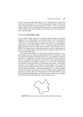
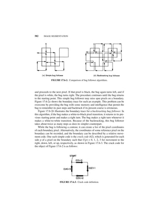
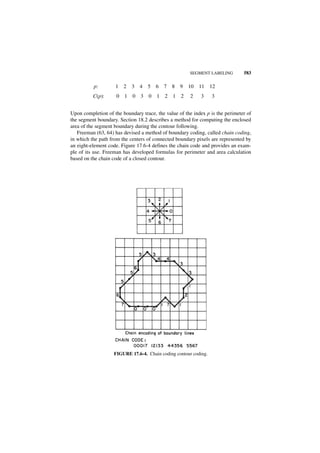
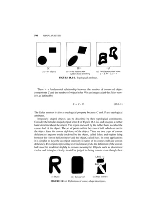
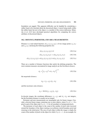
This document provides a summary of the third edition of the textbook "Digital Image Processing: PIKS Inside" by William K. Pratt. The book covers topics related to digital image processing, including continuous and discrete image characterization, linear processing techniques, image improvement, analysis, and software. It is copyrighted in 2001 by John Wiley and Sons and has ISBN numbers for both the hardback and electronic versions.


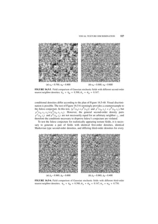
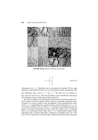
![TWO-DIMENSIONAL FOURIER TRANSFORM 11
F ( ω x, ω y ) = O F { F ( x, y ) } (1.3-2)
In general, the Fourier coefficient F ( ω x, ω y ) is a complex number that may be rep-
resented in real and imaginary form,
F ( ω x, ω y ) = R ( ω x, ω y ) + iI ( ω x, ω y ) (1.3-3a)
or in magnitude and phase-angle form,
F ( ω x, ω y ) = M ( ω x, ω y ) exp { iφ ( ω x, ω y ) } (1.3-3b)
where
2 2 1⁄2
M ( ω x, ω y ) = [ R ( ω x, ω y ) + I ( ω x, ω y ) ] (1.3-4a)
I ( ω x, ω y )
φ ( ω x, ω y ) = arc tan -----------------------
- (1.3-4b)
R ( ω x, ω y )
A sufficient condition for the existence of the Fourier transform of F(x, y) is that the
function be absolutely integrable. That is,
∞ ∞
∫–∞ ∫–∞ F ( x, y ) dx dy < ∞ (1.3-5)
The input function F(x, y) can be recovered from its Fourier transform by the inver-
sion formula
1- ∞ ∞
F ( x, y ) = -------- ∫ ∫ F ( ω x, ω y ) exp { i ( ω x x + ω y y ) } dω x dω y (1.3-6a)
2
4π –∞ – ∞
or in operator form
–1
F ( x, y ) = O F { F ( ω x, ω y ) } (1.3-6b)
The functions F(x, y) and F ( ω x, ω y ) are called Fourier transform pairs.](https://image.slidesharecdn.com/digitalimageprocessing-120319064358-phpapp01/85/Digital-image-processing-25-320.jpg)

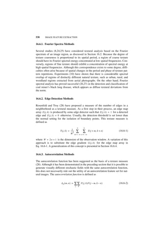
![IMAGE STOCHASTIC CHARACTERIZATION 15
Equations 1.3-20 and 1.3-24 represent two alternative means of determining the out-
put image response of an additive, linear, space-invariant system. The analytic or
operational choice between the two approaches, convolution or Fourier processing,
is usually problem dependent.
1.4. IMAGE STOCHASTIC CHARACTERIZATION
The following presentation on the statistical characterization of images assumes
general familiarity with probability theory, random variables, and stochastic pro-
cess. References 2 and 4 to 7 can provide suitable background. The primary purpose
of the discussion here is to introduce notation and develop stochastic image models.
It is often convenient to regard an image as a sample of a stochastic process. For
continuous images, the image function F(x, y, t) is assumed to be a member of a con-
tinuous three-dimensional stochastic process with space variables (x, y) and time
variable (t).
The stochastic process F(x, y, t) can be described completely by knowledge of its
joint probability density
p { F 1, F2 …, F J ; x 1, y 1, t 1, x 2, y 2, t 2, …, xJ , yJ , tJ }
for all sample points J, where (xj, yj, tj) represent space and time samples of image
function Fj(xj, yj, tj). In general, high-order joint probability densities of images are
usually not known, nor are they easily modeled. The first-order probability density
p(F; x, y, t) can sometimes be modeled successfully on the basis of the physics of
the process or histogram measurements. For example, the first-order probability
density of random noise from an electronic sensor is usually well modeled by a
Gaussian density of the form
2
2 –1 ⁄ 2 [ F ( x, y, t ) – η F ( x, y, t ) ]
p { F ; x, y, t} = [ 2πσ F ( x, y, t ) ] exp – -----------------------------------------------------------
- (1.4-1)
2
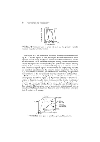
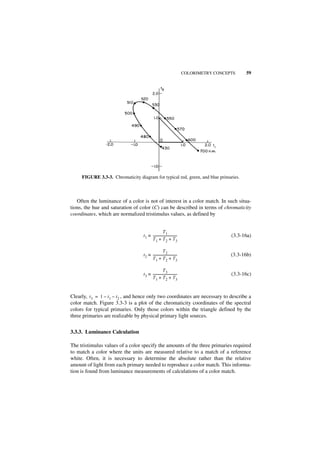
2σ F ( x, y, t )
2
where the parameters η F ( x, y, t ) and σ F ( x, y, t ) denote the mean and variance of the
process. The Gaussian density is also a reasonably accurate model for the probabil-
ity density of the amplitude of unitary transform coefficients of an image. The
probability density of the luminance function must be a one-sided density because
the luminance measure is positive. Models that have found application include the
Rayleigh density,
F ( x, y, t ) [ F ( x, y, t ) ] 2
p { F ; x, y, t } = --------------------- exp – ----------------------------
- (1.4-2a)
2 2
α 2α
the log-normal density,](https://image.slidesharecdn.com/digitalimageprocessing-120319064358-phpapp01/85/Digital-image-processing-29-320.jpg)
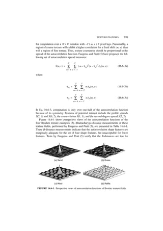
![16 CONTINUOUS IMAGE MATHEMATICAL CHARACTERIZATION
2
2 2 –1 ⁄ 2 [ log { F ( x, y, t ) } – η F ( x, y, t ) ]
p { F ; x, y, t} = [ 2πF ( x, y, t )σ F ( x, y, t ) ] exp – --------------------------------------------------------------------------
-
2
2σ F ( x, y, t )
(1.4-2b)
and the exponential density,
p {F ; x, y, t} = α exp{ – α F ( x, y, t ) } (1.4-2c)
all defined for F ≥ 0, where α is a constant. The two-sided, or Laplacian density,
α
p { F ; x, y, t} = --- exp{ – α F ( x, y, t ) } (1.4-3)
2
where α is a constant, is often selected as a model for the probability density of the
difference of image samples. Finally, the uniform density
1
p { F ; x, y, t} = -----
- (1.4-4)
2π
for – π ≤ F ≤ π is a common model for phase fluctuations of a random process. Con-
ditional probability densities are also useful in characterizing a stochastic process.
The conditional density of an image function evaluated at ( x 1, y 1, t 1 ) given knowl-
edge of the image function at ( x 2, y 2, t 2 ) is defined as
p { F 1, F 2 ; x 1, y 1, t 1, x 2, y 2, t 2}
p { F 1 ; x 1, y 1, t 1 F2 ; x 2, y 2, t 2} = ------------------------------------------------------------------------ (1.4-5)
p { F 2 ; x 2, y 2, t2}
Higher-order conditional densities are defined in a similar manner.
Another means of describing a stochastic process is through computation of its
ensemble averages. The first moment or mean of the image function is defined as
∞
η F ( x, y, t ) = E { F ( x, y, t ) } = ∫– ∞ F ( x, y, t )p { F ; x, y, t} dF (1.4-6)
where E { · } is the expectation operator, as defined by the right-hand side of Eq.
1.4-6.
The second moment or autocorrelation function is given by
R ( x 1, y 1, t 1 ; x 2, y 2, t 2) = E { F ( x 1, y 1, t 1 )F ∗ ( x 2, y 2, t 2 ) } (1.4-7a)
or in explicit form](https://image.slidesharecdn.com/digitalimageprocessing-120319064358-phpapp01/85/Digital-image-processing-30-320.jpg)
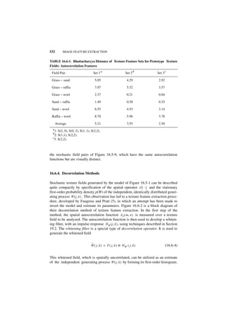
![IMAGE STOCHASTIC CHARACTERIZATION 17
∞ ∞
R ( x 1, y 1, t 1 ; x 2, y 2, t2 ) = ∫–∞ ∫–∞ F ( x1, x1, y1 )F∗ ( x2, y2, t2 )
× p { F 1, F 2 ; x 1, y 1, t1, x 2, y 2, t 2 } dF 1 dF2 (1.4-7b)
The autocovariance of the image process is the autocorrelation about the mean,
defined as
K ( x1, y 1, t1 ; x 2, y 2, t2) = E { [ F ( x 1, y 1, t1 ) – η F ( x 1, y 1, t 1 ) ] [ F∗ ( x 2, y 2, t 2 ) – η∗ ( x 2, y 2, t2 ) ] }
F
(1.4-8a)
or
K ( x 1, y 1, t 1 ; x 2, y 2, t2) = R ( x1, y 1, t1 ; x 2, y 2, t2) – η F ( x 1, y 1, t1 ) η∗ ( x 2, y 2, t 2 )
F (1.4-8b)
Finally, the variance of an image process is
2
σ F ( x, y, t ) = K ( x, y, t ; x, y, t ) (1.4-9)
An image process is called stationary in the strict sense if its moments are unaf-
fected by shifts in the space and time origins. The image process is said to be sta-
tionary in the wide sense if its mean is constant and its autocorrelation is dependent
on the differences in the image coordinates, x1 – x2, y1 – y2, t1 – t2, and not on their
individual values. In other words, the image autocorrelation is not a function of
position or time. For stationary image processes,
E { F ( x, y, t ) } = η F (1.4-10a)
R ( x 1, y 1, t 1 ; x 2, y 2, t 2) = R ( x1 – x 2, y 1 – y 2, t1 – t 2 ) (1.4-10b)
The autocorrelation expression may then be written as
R ( τx, τy, τt ) = E { F ( x + τ x, y + τy, t + τ t )F∗ ( x, y, t ) } (1.4-11)](https://image.slidesharecdn.com/digitalimageprocessing-120319064358-phpapp01/85/Digital-image-processing-31-320.jpg)
![18 CONTINUOUS IMAGE MATHEMATICAL CHARACTERIZATION
Because
R ( – τx, – τ y, – τ t ) = R∗ ( τx, τy, τt ) (1.4-12)
then for an image function with F real, the autocorrelation is real and an even func-
tion of τ x, τ y, τ t . The power spectral density, also called the power spectrum, of a
stationary image process is defined as the three-dimensional Fourier transform of its
autocorrelation function as given by
∞ ∞ ∞
W ( ω x, ω y, ω t ) = ∫–∞ ∫–∞ ∫–∞ R ( τx, τy, τt ) exp { –i ( ωx τx + ωy τy + ω t τt ) } dτx dτy dτt
(1.4-13)
In many imaging systems, the spatial and time image processes are separable so
that the stationary correlation function may be written as
R ( τx, τy, τt ) = R xy ( τx, τy )Rt ( τ t ) (1.4-14)
Furthermore, the spatial autocorrelation function is often considered as the product
of x and y axis autocorrelation functions,
R xy ( τ x, τ y ) = Rx ( τ x )R y ( τ y ) (1.4-15)
for computational simplicity. For scenes of manufactured objects, there is often a
large amount of horizontal and vertical image structure, and the spatial separation
approximation may be quite good. In natural scenes, there usually is no preferential
direction of correlation; the spatial autocorrelation function tends to be rotationally
symmetric and not separable.
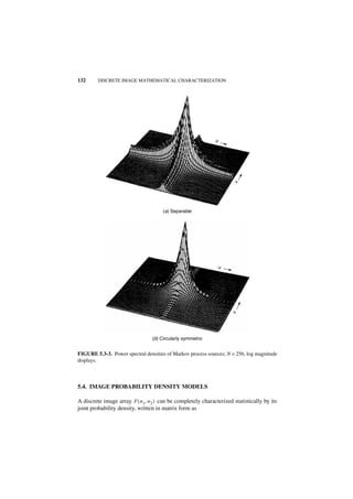
An image field is often modeled as a sample of a first-order Markov process for
which the correlation between points on the image field is proportional to their geo-
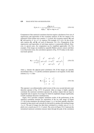
metric separation. The autocovariance function for the two-dimensional Markov
process is
2 2 2 2
R xy ( τ x, τ y ) = C exp – α x τ x + α y τ y (1.4-16)
where C is an energy scaling constant and α x and α y are spatial scaling constants.
The corresponding power spectrum is
1 - 2C
W ( ω x, ω y ) = --------------- -----------------------------------------------------
- (1.4-17)
α x αy 1 + [ ωx ⁄ α2 + ω2 ⁄ α2 ]
2
x y y](https://image.slidesharecdn.com/digitalimageprocessing-120319064358-phpapp01/85/Digital-image-processing-32-320.jpg)


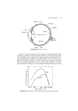

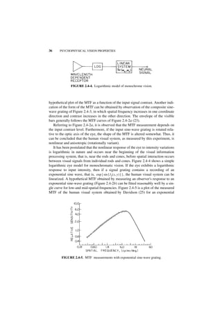
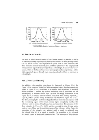
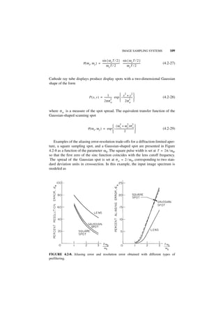
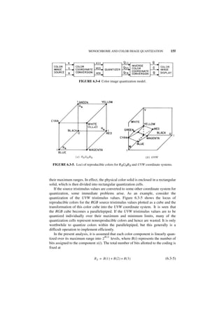
![MONOCHROME VISION MODEL 37
sine-wave test signal. The high-spatial-frequency portion of the curve has been
extrapolated for an average input contrast.
The logarithmic/linear system eye model of Figure 2.4-4 has proved to provide a
reasonable prediction of visual response over a wide range of intensities. However,
at high spatial frequencies and at very low or very high intensities, observed
responses depart from responses predicted by the model. To establish a more accu-
rate model, it is necessary to consider the physical mechanisms of the human visual
system.
The nonlinear response of rods and cones to intensity variations is still a subject
of active research. Hypotheses have been introduced suggesting that the nonlinearity
is based on chemical activity, electrical effects, and neural feedback. The basic loga-
rithmic model assumes the form
IO ( x, y ) = K 1 log { K 2 + K 3 I I ( x, y ) } (2.4-6)
where the Ki are constants and I I ( x, y ) denotes the input field to the nonlinearity
and I O ( x, y ) is its output. Another model that has been suggested (7, p. 253) follows
the fractional response
K 1 I I ( x, y )
I O ( x, y ) = -----------------------------
- (2.4-7)
K 2 + I I ( x, y )
where K 1 and K 2 are constants. Mannos and Sakrison (26) have studied the effect
of various nonlinearities employed in an analytical visual fidelity measure. Their
results, which are discussed in greater detail in Chapter 3, establish that a power law
nonlinearity of the form
s
I O ( x, y ) = [ I I ( x, y ) ] (2.4-8)
where s is a constant, typically 1/3 or 1/2, provides good agreement between the
visual fidelity measure and subjective assessment. The three models for the nonlin-
ear response of rods and cones defined by Eqs. 2.4-6 to 2.4-8 can be forced to a
reasonably close agreement over some midintensity range by an appropriate choice
of scaling constants.
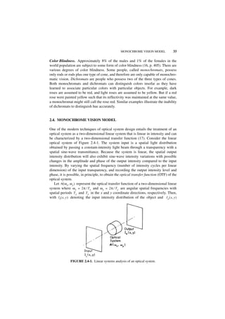
The physical mechanisms accounting for the spatial frequency response of the eye
are partially optical and partially neural. As an optical instrument, the eye has limited
resolution because of the finite size of the lens aperture, optical aberrations, and the
finite dimensions of the rods and cones. These effects can be modeled by a low-pass
transfer function inserted between the receptor and the nonlinear response element.
The most significant contributor to the frequency response of the eye is the lateral
inhibition process (27). The basic mechanism of lateral inhibition is illustrated in](https://image.slidesharecdn.com/digitalimageprocessing-120319064358-phpapp01/85/Digital-image-processing-50-320.jpg)
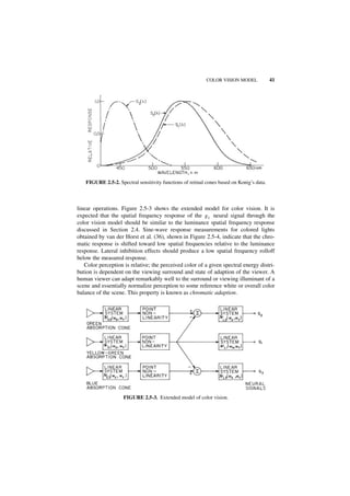
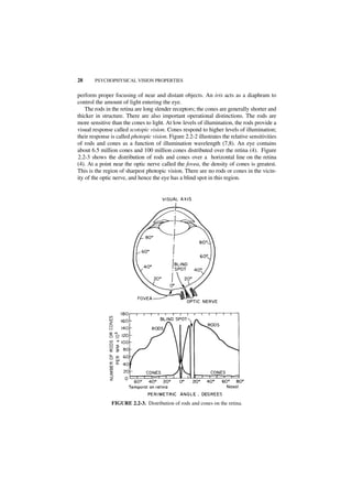
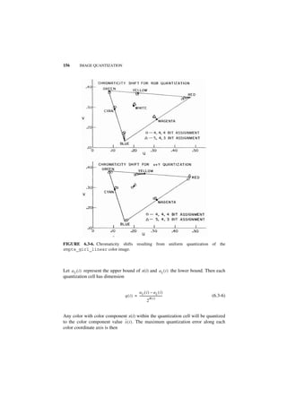
![42 PSYCHOPHYSICAL VISION PROPERTIES
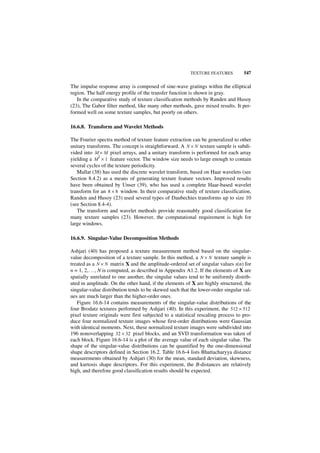
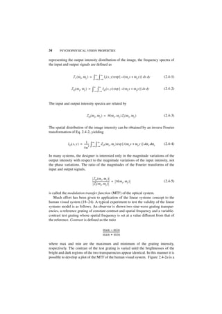
FIGURE 2.5-4. Spatial frequency response measurements of the human visual system.
The simplest visual model for chromatic adaption, proposed by von Kries (37,
16, p. 435), involves the insertion of automatic gain controls between the cones and
first linear system of Figure 2.5-2. These gains
–1
ai = [ ∫ W ( λ )si ( λ ) dλ] (2.5-3)
for i = 1, 2, 3 are adjusted such that the modified cone response is unity when view-
ing a reference white with spectral energy distribution W ( λ ) . Von Kries's model is
attractive because of its qualitative reasonableness and simplicity, but chromatic
testing (16, p. 438) has shown that the model does not completely predict the chro-
matic adaptation effect. Wallis (38) has suggested that chromatic adaption may, in
part, result from a post-retinal neural inhibition mechanism that linearly attenuates
slowly varying visual field components. The mechanism could be modeled by the
low-spatial-frequency attenuation associated with the post-retinal transfer functions
H Li ( ω x, ω y ) of Figure 2.5-3. Undoubtedly, both retinal and post-retinal mechanisms
are responsible for the chromatic adaption effect. Further analysis and testing are
required to model the effect adequately.
REFERENCES
1. Webster's New Collegiate Dictionary, G. & C. Merriam Co. (The Riverside Press),
Springfield, MA, 1960.
2. H. H. Malitson, “The Solar Energy Spectrum,” Sky and Telescope, 29, 4, March 1965,
162–165.
3. Munsell Book of Color, Munsell Color Co., Baltimore.
4. M. H. Pirenne, Vision and the Eye, 2nd ed., Associated Book Publishers, London, 1967.
5. S. L. Polyak, The Retina, University of Chicago Press, Chicago, 1941.](https://image.slidesharecdn.com/digitalimageprocessing-120319064358-phpapp01/85/Digital-image-processing-55-320.jpg)


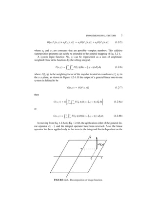
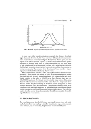
![Digital Image Processing: PIKS Inside, Third Edition. William K. Pratt
Copyright © 2001 John Wiley & Sons, Inc.
ISBNs: 0-471-37407-5 (Hardback); 0-471-22132-5 (Electronic)
3
PHOTOMETRY AND COLORIMETRY
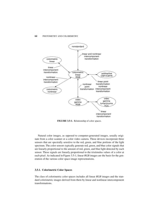
Chapter 2 dealt with human vision from a qualitative viewpoint in an attempt to
establish models for monochrome and color vision. These models may be made
quantitative by specifying measures of human light perception. Luminance mea-
sures are the subject of the science of photometry, while color measures are treated
by the science of colorimetry.
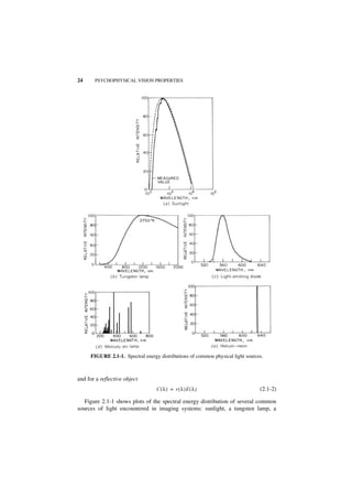
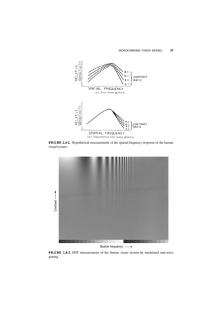
3.1. PHOTOMETRY
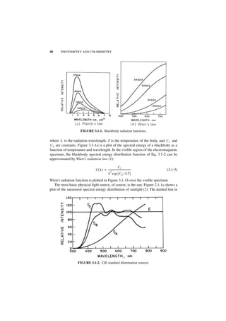
A source of radiative energy may be characterized by its spectral energy distribution
C ( λ ) , which specifies the time rate of energy the source emits per unit wavelength
interval. The total power emitted by a radiant source, given by the integral of the
spectral energy distribution,
∞
P = ∫0 C(λ ) d λ (3.1-1)
is called the radiant flux of the source and is normally expressed in watts (W).
A body that exists at an elevated temperature radiates electromagnetic energy
proportional in amount to its temperature. A blackbody is an idealized type of heat
radiator whose radiant flux is the maximum obtainable at any wavelength for a body
at a fixed temperature. The spectral energy distribution of a blackbody is given by
Planck's law (1):
C1
C ( λ ) = ----------------------------------------------------- (3.1-2)
5
λ [ exp { C 2 ⁄ λT } – 1 ]
45](https://image.slidesharecdn.com/digitalimageprocessing-120319064358-phpapp01/85/Digital-image-processing-58-320.jpg)
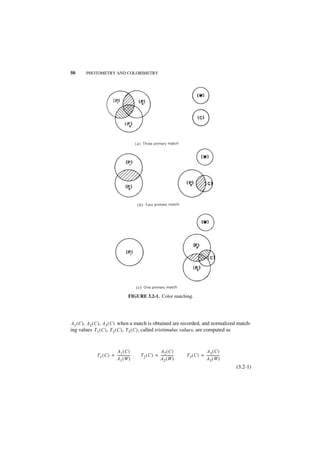
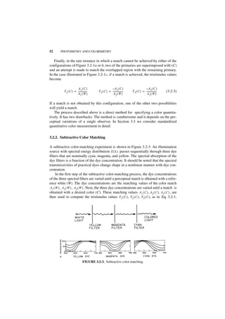
![COLOR MATCHING 53
It should be apparent that there is no fundamental theoretical difference between
color matching by an additive or a subtractive system. In a subtractive system, the
yellow dye acts as a variable absorber of blue light, and with ideal dyes, the yellow
dye effectively forms a blue primary light. In a similar manner, the magenta filter
ideally forms the green primary, and the cyan filter ideally forms the red primary.
Subtractive color systems ordinarily utilize cyan, magenta, and yellow dye spectral
filters rather than red, green, and blue dye filters because the cyan, magenta, and
yellow filters are notch filters which permit a greater transmission of light energy
than do narrowband red, green, and blue bandpass filters. In color printing, a fourth
filter layer of variable gray level density is often introduced to achieve a higher con-
trast in reproduction because common dyes do not possess a wide density range.
3.2.3. Axioms of Color Matching
The color-matching experiments described for additive and subtractive color match-
ing have been performed quite accurately by a number of researchers. It has been
found that perfect color matches sometimes cannot be obtained at either very high or
very low levels of illumination. Also, the color matching results do depend to some
extent on the spectral composition of the surrounding light. Nevertheless, the simple
color matching experiments have been found to hold over a wide range of condi-
tions.
Grassman (15) has developed a set of eight axioms that define trichromatic color
matching and that serve as a basis for quantitative color measurements. In the
following presentation of these axioms, the symbol ◊ indicates a color match; the
symbol ⊕ indicates an additive color mixture; the symbol • indicates units of a
color. These axioms are:
1. Any color can be matched by a mixture of no more than three colored lights.
2. A color match at one radiance level holds over a wide range of levels.
3. Components of a mixture of colored lights cannot be resolved by the human eye.
4. The luminance of a color mixture is equal to the sum of the luminance of its
components.
5. Law of addition. If color (M) matches color (N) and color (P) matches color (Q),
then color (M) mixed with color (P) matches color (N) mixed with color (Q):
( M ) ◊ ( N ) ∩ ( P ) ◊ ( Q) ⇒ [ ( M) ⊕ ( P) ] ◊ [ ( N ) ⊕ ( Q )] (3.2-4)
6. Law of subtraction. If the mixture of (M) plus (P) matches the mixture of (N)
plus (Q) and if (P) matches (Q), then (M) matches (N):
[ (M ) ⊕ (P )] ◊ [(N ) ⊕ ( Q) ] ∩ [( P) ◊ (Q) ] ⇒ ( M) ◊ (N ) (3.2-5)
7. Transitive law. If (M) matches (N) and if (N) matches (P), then (M) matches (P):](https://image.slidesharecdn.com/digitalimageprocessing-120319064358-phpapp01/85/Digital-image-processing-66-320.jpg)
![54 PHOTOMETRY AND COLORIMETRY
[ (M) ◊ (N)] ∩ [(N) ◊ (P) ] ⇒ (M) ◊ (P) (3.2-6)
8. Color matching. (a) c units of (C) matches the mixture of m units of (M) plus n
units of (N) plus p units of (P):
c • C ◊ [m • (M )] ⊕ [n • ( N) ] ⊕ [p • (P ) ] (3.2-7)
or (b) a mixture of c units of C plus m units of M matches the mixture of n units
of N plus p units of P:
[c • (C )] ⊕ [m • ( M) ] ◊ [n • (N)] ⊕ [ p • (P) ] (3.2-8)
or (c) a mixture of c units of (C) plus m units of (M) plus n units of (N) matches p
units of P:
[c • (C )] ⊕ [m • ( M) ] ⊕ [n • (N )] ◊ [ p • (P) ] (3.2-9)
With Grassman's laws now specified, consideration is given to the development of a
quantitative theory for color matching.
3.3. COLORIMETRY CONCEPTS
Colorimetry is the science of quantitatively measuring color. In the trichromatic
color system, color measurements are in terms of the tristimulus values of a color or
a mathematical function of the tristimulus values.
Referring to Section 3.2.3, the axioms of color matching state that a color C can
be matched by three primary colors P1, P2, P3. The qualitative match is expressed as
( C ) ◊ [ A 1 ( C ) • ( P 1 ) ] ⊕ [ A 2 ( C ) • ( P 2 ) ] ⊕ [ A3 ( C ) • ( P 3 ) ] (3.3-1)
where A 1 ( C ) , A2 ( C ) , A 3 ( C ) are the matching values of the color (C). Because the
intensities of incoherent light sources add linearly, the spectral energy distribution of
a color mixture is equal to the sum of the spectral energy distributions of its compo-
nents. As a consequence of this fact and Eq. 3.3-1, the spectral energy distribution
C ( λ ) can be replaced by its color-matching equivalent according to the relation
3
C ( λ ) ◊ A 1 ( C )P 1 ( λ ) + A2 ( C )P2 ( λ ) + A 3 ( C )P 3 ( λ ) = ∑ A j ( C )Pj ( λ ) (3.3-2)
j =1](https://image.slidesharecdn.com/digitalimageprocessing-120319064358-phpapp01/85/Digital-image-processing-67-320.jpg)

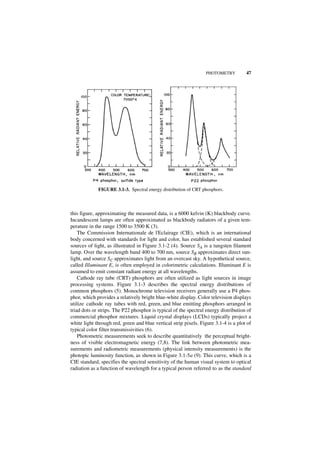
![56 PHOTOMETRY AND COLORIMETRY
If a viewer observes the primary mixture instead of C, then from Eq. 3.3-4, substitu-
tion for C ( λ ) should result in the same cone signals e i ( C ) . Thus
3
e1 ( C ) = ∑ Tj ( C )Aj ( W ) ∫ Pj ( λ )s1 ( λ ) d λ (3.3-7a)
j =1
3
e2( C ) = ∑ Tj ( C )Aj ( W ) ∫ Pj ( λ )s2 ( λ ) d λ (3.3-7b)
j =1
3
e3 ( C ) = ∑ Tj ( C )Aj ( W ) ∫ Pj ( λ )s3 ( λ ) d λ (3.3-7c)
j =1
Equation 3.3-7 can be written more compactly in matrix form by defining
k ij = ∫ Pj ( λ )si ( λ ) dλ (3.3-8)
Then
e1 ( C ) k 11 k 12 k 13 A1( W ) 0 0 T1 ( C )
e2 ( C ) = k 21 k 22 k 23 0 A2( W ) 0 T2 ( C ) (3.3-9)
e3 ( C ) k 31 k 32 k 33 0 0 A3( W ) T3 ( C )
or in yet more abbreviated form,
e ( C ) = KAt ( C ) (3.3-10)
where the vectors and matrices of Eq. 3.3-10 are defined in correspondence with
Eqs. 3.3-7 to 3.3-9. The vector space notation used in this section is consistent with
the notation formally introduced in Appendix 1. Matrices are denoted as boldface
uppercase symbols, and vectors are denoted as boldface lowercase symbols. It
should be noted that for a given set of primaries, the matrix K is constant valued,
and for a given reference white, the white matching values of the matrix A are con-
stant. Hence, if a set of cone signals e i ( C ) were known for a color (C), the corre-
sponding tristimulus values Tj ( C ) could in theory be obtained from
–1
t ( C ) = [ KA ] e ( C ) (3.3-11)](https://image.slidesharecdn.com/digitalimageprocessing-120319064358-phpapp01/85/Digital-image-processing-69-320.jpg)
![COLORIMETRY CONCEPTS 57
provided that the matrix inverse of [KA] exists. Thus, it has been shown that with
proper selection of the tristimulus signals Tj ( C ) , any color can be matched in the
sense that the cone signals will be the same for the primary mixture as for the actual
color C. Unfortunately, the cone signals e i ( C ) are not easily measured physical
quantities, and therefore, Eq. 3.3-11 cannot be used directly to compute the tristimu-
lus values of a color. However, this has not been the intention of the derivation.
Rather, Eq. 3.3-11 has been developed to show the consistency of the color-match-
ing experiment with the color vision model.
3.3.2. Tristimulus Value Calculation
It is possible indirectly to compute the tristimulus values of an arbitrary color for a
particular set of primaries if the tristimulus values of the spectral colors (narrow-
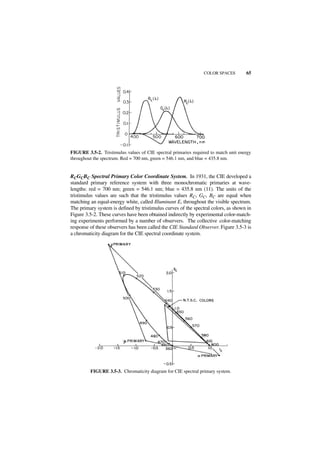
band light) are known for that set of primaries. Figure 3.3-1 is a typical sketch of the
tristimulus values required to match a unit energy spectral color with three arbitrary
primaries. These tristimulus values, which are fundamental to the definition of a pri-
mary system, are denoted as Ts1 ( λ ) , T s2 ( λ ) , T s3 ( λ ) , where λ is a particular wave-
length in the visible region. A unit energy spectral light ( C ψ ) at wavelength ψ with
energy distribution δ ( λ – ψ ) is matched according to the equation
3
e i ( Cψ ) = ∫ δ ( λ – ψ )si ( λ ) d λ = ∑ ∫ Aj ( W )Pj ( λ )Ts ( ψ )si ( λ ) d λ
j
(3.3-12)
j=1
Now, consider an arbitrary color [C] with spectral energy distribution C ( λ ) . At
wavelength ψ , C ( ψ ) units of the color are matched by C ( ψ )Ts1 ( ψ ) , C ( ψ )Ts2 ( ψ ) ,
C ( ψ )T s ( ψ ) tristimulus units of the primaries as governed by
3
3
∫ C ( ψ )δ ( λ – ψ )si ( λ ) d λ = ∑ ∫ Aj ( W )Pj ( λ )C ( ψ )Ts ( ψ )si ( λ ) d λ
j
(3.3-13)
j =1
Integrating each side of Eq. 3.3-13 over ψ and invoking the sifting integral gives the
cone signal for the color (C). Thus
3
∫ ∫ C ( ψ )δ ( λ – ψ )si ( λ ) d λ dψ = ei ( C ) = ∑ ∫ ∫ Aj ( W )Pj ( λ )C ( ψ )Ts ( ψ )si ( λ ) dψ d λ
j
j =1
(3.3-14)
By correspondence with Eq. 3.3-7, the tristimulus values of (C) must be equivalent
to the second integral on the right of Eq. 3.3-14. Hence
Tj ( C ) = ∫ C ( ψ )Ts ( ψ ) dψ
j
(3.3-15)](https://image.slidesharecdn.com/digitalimageprocessing-120319064358-phpapp01/85/Digital-image-processing-70-320.jpg)


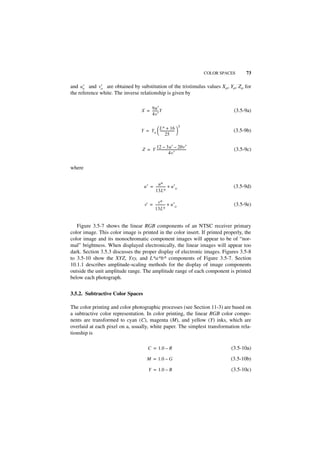
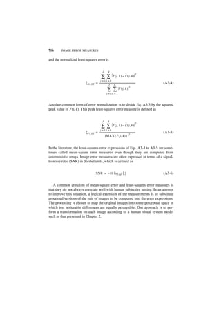
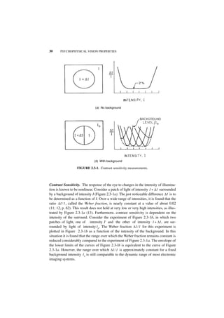
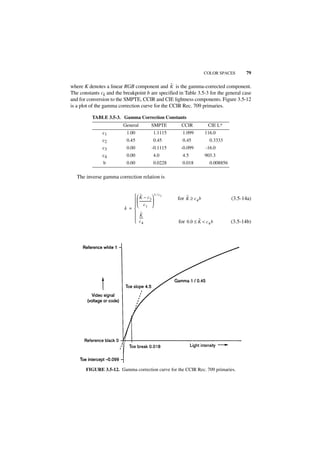
![74 PHOTOMETRY AND COLORIMETRY
(a) Linear R, 0.000 to 0.965
(b) Linear G, 0.000 to 1.000 (c) Linear B, 0.000 to 0.965
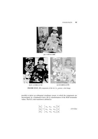
FIGURE 3.5-7. Linear RGB components of the dolls_linear color image. See insert
for a color representation of this figure.
where the linear RGB components are tristimulus values over [0.0, 1.0]. The inverse
relations are
R = 1.0 – C (3.5-11a)
G = 1.0 – M (3.5-11b)
B = 1.0 – Y (3.5-11c)
In high-quality printing systems, the RGB-to-CMY transformations, which are usu-
ally proprietary, involve color component cross-coupling and point nonlinearities.](https://image.slidesharecdn.com/digitalimageprocessing-120319064358-phpapp01/85/Digital-image-processing-87-320.jpg)


![IMAGE SAMPLING SYSTEMS 101
S ( x, y ) = D T ( x, y ) ᭺ P ( x, y )
* (4.2-4)
where
J K
D T ( x, y ) = ∑ ∑ δ ( x – j ∆x, y – k ∆y) (4.2-5)
j = –J k = –K
Combining Eqs. 4.2-1 and 4.2-2 results in an expression for the sampled image
function,
J K
F P ( x, y ) = ∑ ∑ F I ( j ∆x, k ∆ y)P ( x – j ∆x, y – k ∆y) (4.2-6)
j = – J k = –K
The spectrum of the sampled image function is given by
1
F P ( ω x, ω y ) = -------- F I ( ω x, ω y ) ᭺ [ D T ( ω x, ω y )P ( ω x, ω y ) ]
- * (4.2-7)
2
4π
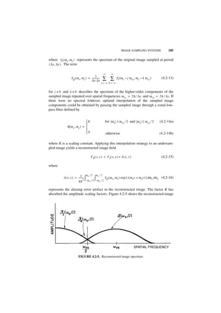
where P ( ω x, ω y ) is the Fourier transform of P ( x, y ) . The Fourier transform of the
truncated sampling array is found to be (5, p. 105)
sin ω x ( J + 1 ) ∆ x sin ω y ( K + 1 ) ∆ y
--
- --
-
2 2
D T ( ω x, ω y ) = --------------------------------------------- ----------------------------------------------
- (4.2-8)
sin { ω x ∆x ⁄ 2 } sin { ω y ∆ y ⁄ 2 }
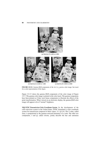
Figure 4.2-2 depicts D T ( ω x, ω y ) . In the limit as J and K become large, the right-hand
side of Eq. 4.2-7 becomes an array of Dirac delta functions.
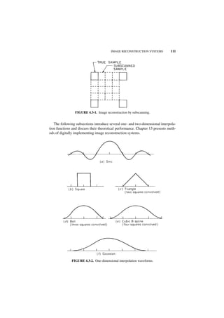
FIGURE 4.2-2. Truncated sampling train and its Fourier spectrum.](https://image.slidesharecdn.com/digitalimageprocessing-120319064358-phpapp01/85/Digital-image-processing-113-320.jpg)
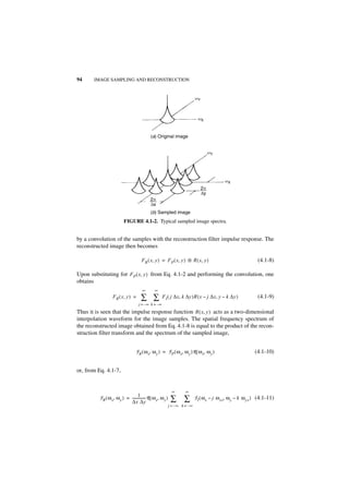
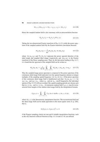
![102 IMAGE SAMPLING AND RECONSTRUCTION
In an image reconstruction system, an image is reconstructed by interpolation of
its samples. Ideal interpolation waveforms such as the sinc function of Eq. 4.1-14 or
the Bessel function of Eq. 4.1-16 generally extend over the entire image field. If the
sampling array is truncated, the reconstructed image will be in error near its bound-
ary because the tails of the interpolation waveforms will be truncated in the vicinity
of the boundary (8,9). However, the error is usually negligibly small at distances of
about 8 to 10 Nyquist samples or greater from the boundary.
The actual numerical samples of an image are obtained by a spatial integration of
FS ( x, y ) over some finite resolution cell. In the scanning system of Figure 4.2-1, the
integration is inherently performed on the photodetector surface. The image sample
value of the resolution cell (j, k) may then be expressed as
j∆x + A x k∆y + A y
F S ( j ∆x, k ∆y) = ∫j∆x – A ∫k∆y – A
x y
F I ( x, y )P ( x – j ∆x, y – k ∆y ) dx dy (4.2-9)
where Ax and Ay denote the maximum dimensions of the resolution cell. It is
assumed that only one sample pulse exists during the integration time of the detec-
tor. If this assumption is not valid, consideration must be given to the difficult prob-
lem of sample crosstalk. In the sampling system under discussion, the width of the
resolution cell may be larger than the sample spacing. Thus the model provides for
sequentially overlapped samples in time.
By a simple change of variables, Eq. 4.2-9 may be rewritten as
Ax Ay
FS ( j ∆x, k ∆y) = ∫–A ∫–A FI ( j ∆x – α, k ∆y – β )P ( – α, – β ) dx dy
x y
(4.2-10)
Because only a single sampling pulse is assumed to occur during the integration
period, the limits of Eq. 4.2-10 can be extended infinitely . In this formulation, Eq.
4.2-10 is recognized to be equivalent to a convolution of the ideal continuous image
FI ( x, y ) with an impulse response function P ( – x, – y ) with reversed coordinates,
followed by sampling over a finite area with Dirac delta functions. Thus, neglecting
the effects of the finite size of the sampling array, the model for finite extent pulse
sampling becomes
F S ( j ∆x, k ∆y) = [ FI ( x, y ) ᭺ P ( – x, – y ) ]δ ( x – j ∆x, y – k ∆y)
* (4.2-11)
In most sampling systems, the sampling pulse is symmetric, so that P ( – x, – y ) = P ( x, y ).
Equation 4.2-11 provides a simple relation that is useful in assessing the effect
of finite extent pulse sampling. If the ideal image is bandlimited and Ax and Ay sat-
isfy the Nyquist criterion, the finite extent of the sample pulse represents an equiv-
alent linear spatial degradation (an image blur) that occurs before ideal sampling.
Part 4 considers methods of compensating for this degradation. A finite-extent
sampling pulse is not always a detriment, however. Consider the situation in which](https://image.slidesharecdn.com/digitalimageprocessing-120319064358-phpapp01/85/Digital-image-processing-114-320.jpg)
![IMAGE SAMPLING SYSTEMS 103
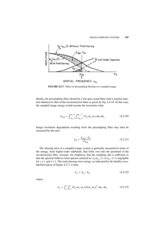
the ideal image is insufficiently bandlimited so that it is undersampled. The finite-
extent pulse, in effect, provides a low-pass filtering of the ideal image, which, in
turn, serves to limit its spatial frequency content, and hence to minimize aliasing
error.
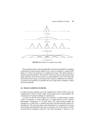
4.2.2. Aliasing Effects
To achieve perfect image reconstruction in a sampled imaging system, it is neces-
sary to bandlimit the image to be sampled, spatially sample the image at the Nyquist
or higher rate, and properly interpolate the image samples. Sample interpolation is
considered in the next section; an analysis is presented here of the effect of under-
sampling an image.
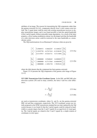
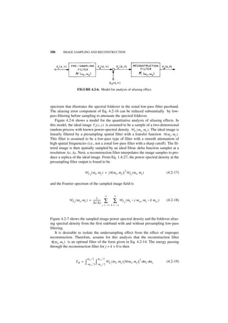
If there is spectral overlap resulting from undersampling, as indicated by the
shaded regions in Figure 4.2-3, spurious spatial frequency components will be intro-
duced into the reconstruction. The effect is called an aliasing error (10,11). Aliasing
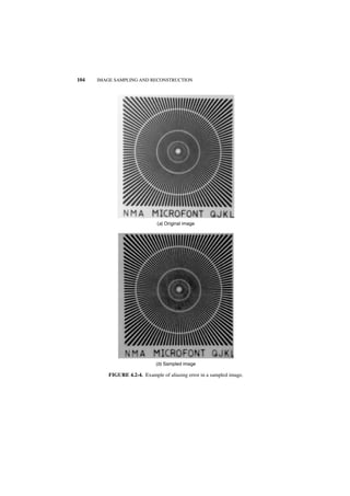
effects in an actual image are shown in Figure 4.2-4. Spatial undersampling of the
image creates artificial low-spatial-frequency components in the reconstruction. In
the field of optics, aliasing errors are called moiré patterns.
From Eq. 4.1-7 the spectrum of a sampled image can be written in the form
1
F P ( ω x, ω y ) = ------------- [ F I ( ω x, ω y ) + F Q ( ω x, ω y ) ] (4.2-12)
∆x ∆y
−
FIGURE 4.2-3. Spectra of undersampled two-dimensional function.](https://image.slidesharecdn.com/digitalimageprocessing-120319064358-phpapp01/85/Digital-image-processing-115-320.jpg)

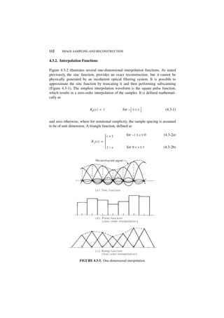
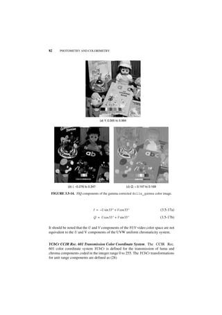
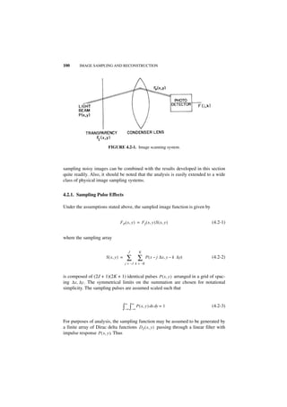
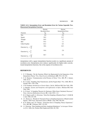
![IMAGE RECONSTRUCTION SYSTEMS 115
TABLE 4.3-1. Two-Dimensional Interpolation Functions
Function Definition
Separable sinc 4 sin { 2πx ⁄ T x } sin { 2πy ⁄ T y } 2π
R ( x, y ) = ---------- --------------------------------- ---------------------------------
- T x = -------
-
T x T y 2πx ⁄ T x 2πy ⁄ T y ω xs
2π
T y = -------
-
ω ys
1 ω x ≤ ω xs , ω y ≤ ω ys
( ω x, ω y ) =
0 otherwise
Separable square
1 Tx Ty
----------
- x ≤ ---- ,
- y ≤ ----
-
R 0 ( x, y ) = T x T y 2 2
0 otherwise
sin { ω x T x ⁄ 2 } sin { ω y T y ⁄ 2 }
0 ( ω x ,ω y ) = -------------------------------------------------------------------
-
( ωx Tx ⁄ 2 ) ( ω y Ty ⁄ 2 )
Separable triangle R 1 ( x, y ) = R 0 ( x, y ) ᭺ R0 ( x, y )
*
2
1 ( ω x, ω y ) = 0 ( ω x, ω y )
Separable bell R 2 ( x, y ) = R 0 ( x, y ) ᭺ R1 ( x, y )
*
3
2 ( ω x, ω y ) = 0 ( ω x, ω y )
Separable cubic B-spline R 3 ( x, y ) = R 0 ( x, y ) ᭺ R2 ( x, y )
*
4
3 ( ω x, ω y ) = 0 ( ω x, ω y )
Gaussian
2 –1 x2 + y2
R ( x, y ) = [ 2πσ w ] exp – ----------------
2σ 3 w
2 2 2
σw ( ωx + ωy )
( ω x, ω y ) = exp – -------------------------------
2
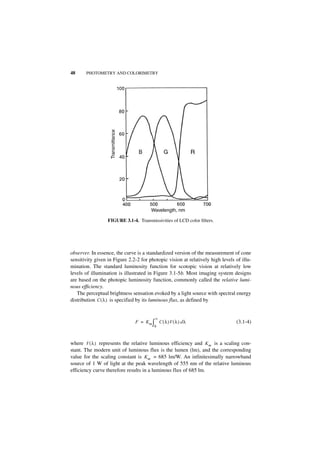
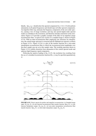
4.3.3. Effect of Imperfect Reconstruction Filters
The performance of practical image reconstruction systems will now be analyzed. It
will be assumed that the input to the image reconstruction system is composed of
samples of an ideal image obtained by sampling with a finite array of Dirac
samples at the Nyquist rate. From Eq. 4.1-9 the reconstructed image is found to be
∞ ∞
F R ( x, y ) = ∑ ∑ F I ( j ∆x, k ∆y)R ( x – j ∆x, y – k ∆y) (4.3-7)
j = –∞ k = –∞](https://image.slidesharecdn.com/digitalimageprocessing-120319064358-phpapp01/85/Digital-image-processing-127-320.jpg)
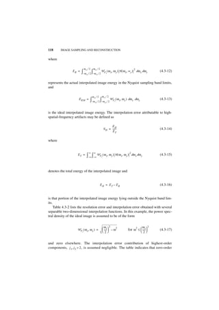
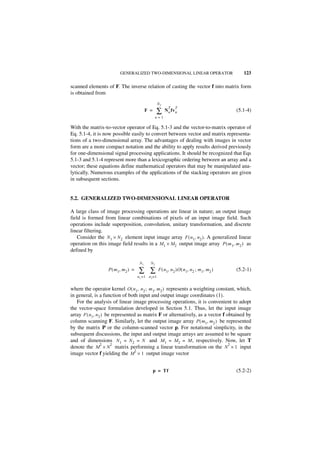
![116 IMAGE SAMPLING AND RECONSTRUCTION
FIGURE 4.3-4. Two-dimensional linear interpolation.
where R(x, y) is the two-dimensional interpolation function of the image reconstruc-
tion system. Ideally, the reconstructed image would be the exact replica of the ideal
image as obtained from Eq. 4.1-9. That is,
∞ ∞
ˆ
F R ( x, y ) = ∑ ∑ F I ( j ∆x, k ∆y)R I ( x – j ∆ x, y – k ∆y) (4.3-8)
j = – ∞ k = –∞
where R I ( x, y ) represents an optimum interpolation function such as given by Eq.
4.1-14 or 4.1-16. The reconstruction error over the bounds of the sampled image is
then
∞ ∞
ED ( x, y ) = ∑ ∑ FI ( j ∆x, k ∆y) [ R ( x – j ∆x, y – k ∆y) – R I ( x – j ∆x, y – k ∆y) ] (4.3-9)
j = –∞ k = – ∞
There are two contributors to the reconstruction error: (1) the physical system
interpolation function R(x, y) may differ from the ideal interpolation function
RI ( x, y ) , and (2) the finite bounds of the reconstruction, which cause truncation of
the interpolation functions at the boundary. In most sampled imaging systems, the
boundary reconstruction error is ignored because the error generally becomes negli-
gible at distances of a few samples from the boundary. The utilization of nonideal
interpolation functions leads to a potential loss of image resolution and to the intro-
duction of high-spatial-frequency artifacts.
The effect of an imperfect reconstruction filter may be analyzed conveniently by
examination of the frequency spectrum of a reconstructed image, as derived in Eq.
4.1-11:
∞ ∞
1
F R ( ω x, ω y ) = -------------- R ( ω x, ω y )
∆x ∆y
- ∑ ∑ F I ( ω x – j ω xs, ω y – k ω ys ) (4.3-10)
j = –∞ k = –∞](https://image.slidesharecdn.com/digitalimageprocessing-120319064358-phpapp01/85/Digital-image-processing-128-320.jpg)

![Digital Image Processing: PIKS Inside, Third Edition. William K. Pratt
Copyright © 2001 John Wiley & Sons, Inc.
ISBNs: 0-471-37407-5 (Hardback); 0-471-22132-5 (Electronic)
5
DISCRETE IMAGE MATHEMATICAL
CHARACTERIZATION
Chapter 1 presented a mathematical characterization of continuous image fields.
This chapter develops a vector-space algebra formalism for representing discrete
image fields from a deterministic and statistical viewpoint. Appendix 1 presents a
summary of vector-space algebra concepts.
5.1. VECTOR-SPACE IMAGE REPRESENTATION
In Chapter 1 a generalized continuous image function F(x, y, t) was selected to
represent the luminance, tristimulus value, or some other appropriate measure of a
physical imaging system. Image sampling techniques, discussed in Chapter 4,
indicated means by which a discrete array F(j, k) could be extracted from the contin-
uous image field at some time instant over some rectangular area – J ≤ j ≤ J ,
– K ≤ k ≤ K . It is often helpful to regard this sampled image array as a N 1 × N 2
element matrix
F = [ F ( n 1, n 2 ) ] (5.1-1)
for 1 ≤ n i ≤ Ni where the indices of the sampled array are reindexed for consistency
with standard vector-space notation. Figure 5.1-1 illustrates the geometric relation-
ship between the Cartesian coordinate system of a continuous image and its array of
samples. Each image sample is called a pixel.
121](https://image.slidesharecdn.com/digitalimageprocessing-120319064358-phpapp01/85/Digital-image-processing-133-320.jpg)

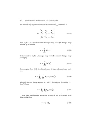
![126 DISCRETE IMAGE MATHEMATICAL CHARACTERIZATION
1. Column processing of F:
T = diag [ T C1, T C2, …, T CN ] (5.2-11)
where T Cj is the transformation matrix for the jth column.
2. Identical column processing of F:
T = diag [ T C, T C, …, T C ] = T C ⊗ I N (5.2-12)
3. Row processing of F:
T mn = diag [ T R1 ( m, n ), T R2 ( m, n ), …, T RN ( m, n ) ] (5.2-13)
where T Rj is the transformation matrix for the jth row.
4. Identical row processing of F:
T mn = diag [ T R ( m, n ), T R ( m, n ), …, T R ( m, n ) ] (5.2-14a)
and
T = IN ⊗ TR (5.2-14b)
5. Identical row and identical column processing of F:
T = TC ⊗ I N + I N ⊗ T R (5.2-15)
The number of computational operations for each of these cases is tabulated in Table
5.2-1.
Equation 5.2-10 indicates that separable two-dimensional linear transforms can
be computed by sequential one-dimensional row and column operations on a data
array. As indicated by Table 5.2-1, a considerable savings in computation is possible
2 2
for such transforms: computation by Eq 5.2-2 in the general case requires M N
2 2
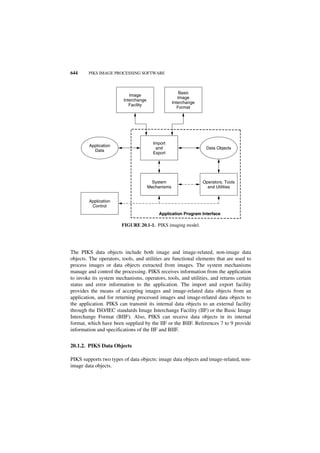
operations; computation by Eq. 5.2-10, when it applies, requires only MN + M N
operations. Furthermore, F may be stored in a serial memory and fetched line by
line. With this technique, however, it is necessary to transpose the result of the col-
umn transforms in order to perform the row transforms. References 2 and 3 describe
algorithms for line storage matrix transposition.](https://image.slidesharecdn.com/digitalimageprocessing-120319064358-phpapp01/85/Digital-image-processing-138-320.jpg)
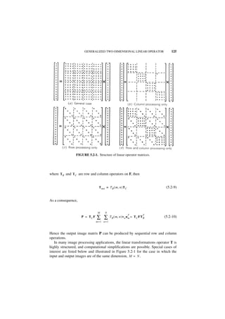
![IMAGE STATISTICAL CHARACTERIZATION 127
TABLE 5.2-1. Computational Requirements for Linear Transform Operator
Operations
Case (Multiply and Add)
General N4
Column processing N3
Row processing N3
Row and column processing 2N3– N2
Separable row and column processing matrix form 2N3
5.3. IMAGE STATISTICAL CHARACTERIZATION
The statistical descriptors of continuous images presented in Chapter 1 can be
applied directly to characterize discrete images. In this section, expressions are
developed for the statistical moments of discrete image arrays. Joint probability
density models for discrete image fields are described in the following section. Ref-
erence 4 provides background information for this subject.
The moments of a discrete image process may be expressed conveniently in
vector-space form. The mean value of the discrete image function is a matrix of the
form
E { F } = [ E { F ( n 1, n 2 ) } ] (5.3-1)
If the image array is written as a column-scanned vector, the mean of the image vec-
tor is
N2
ηf = E { f } = ∑ N n E { F }v n (5.3-2)
n= 1
The correlation function of the image array is given by
R ( n 1, n 2 ; n 3 , n 4 ) = E { F ( n 1, n 2 )F∗ ( n 3, n 4 ) } (5.3-3)
where the n i represent points of the image array. Similarly, the covariance function
of the image array is
K ( n 1, n 2 ; n 3 , n 4) = E { [ F ( n 1, n 2 ) – E { F ( n 1, n 2 ) } ] [ F∗ ( n 3, n 4 ) – E { F∗ ( n 3, n 4 ) } ] }
(5.3-4)](https://image.slidesharecdn.com/digitalimageprocessing-120319064358-phpapp01/85/Digital-image-processing-139-320.jpg)
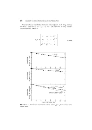
![134 DISCRETE IMAGE MATHEMATICAL CHARACTERIZATION
Probability distributions of image values can be estimated by histogram measure-
ments. For example, the first-order probability distribution
P [ f ( q ) ] = PR [ f ( q ) = r j ] (5.4-6)
of the amplitude value at vector coordinate q can be estimated by examining a large
collection of images representative of a given image class (e.g., chest x-rays, aerial
scenes of crops). The first-order histogram estimate of the probability distribution is
the frequency ratio
Np ( j )
H E ( j ; q ) = -------------
- (5.4-7)
Np
where N p represents the total number of images examined and N p ( j ) denotes the
number for which f ( q ) = r j for j = 0, 1,..., J – 1. If the image source is statistically
stationary, the first-order probability distribution of Eq. 5.4-6 will be the same for all
vector components q. Furthermore, if the image source is ergodic, ensemble aver-
ages (measurements over a collection of pictures) can be replaced by spatial aver-
ages. Under the ergodic assumption, the first-order probability distribution can be
estimated by measurement of the spatial histogram
NS ( j )
HS ( j ) = ------------
- (5.4-8)
Q
where N S ( j ) denotes the number of pixels in an image for which f ( q ) = r j for
1 ≤ q ≤ Q and 0 ≤ j ≤ J – 1 . For example, for an image with 256 gray levels, H S ( j )
denotes the number of pixels possessing gray level j for 0 ≤ j ≤ 255.
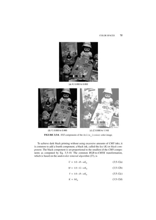
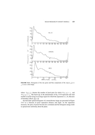
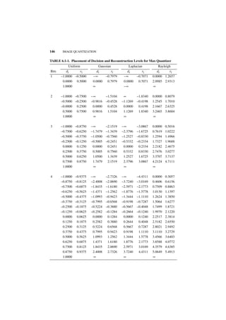
Figure 5.4-1 shows first-order histograms of the red, green, and blue components
of a color image. Most natural images possess many more dark pixels than bright
pixels, and their histograms tend to fall off exponentially at higher luminance levels.
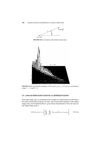
Estimates of the second-order probability distribution for ergodic image sources
can be obtained by measurement of the second-order spatial histogram, which is a
measure of the joint occurrence of pairs of pixels separated by a specified distance.
With reference to Figure 5.4-2, let F ( n1, n 2 ) and F ( n3, n 4 ) denote a pair of pixels
separated by r radial units at an angle θ with respect to the horizontal axis. As a
consequence of the rectilinear grid, the separation parameters may only assume cer-
tain discrete values. The second-order spatial histogram is then the frequency ratio
NS ( j1, j2 )
H S ( j 1, j 2 ; r, θ ) = -----------------------
- (5.4-9)
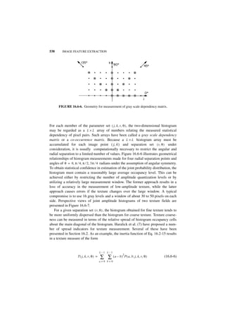
QT](https://image.slidesharecdn.com/digitalimageprocessing-120319064358-phpapp01/85/Digital-image-processing-146-320.jpg)


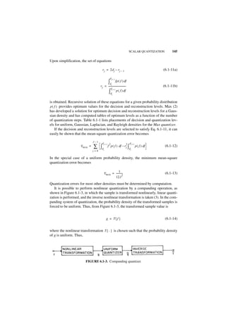
![SCALAR QUANTIZATION 143
FIGURE 6.1-2. Quantization decision and reconstruction levels.
For a large number of quantization levels J, the probability density may be repre-
sented as a constant value p ( r j ) over each quantization band. Hence
J –1
dj + 1 2
E = ∑ p ( r j ) ∫d j
( f – r j ) df (6.1-4)
j= 0
which evaluates to
J–1
1 3 3
E = --
3
- ∑ p ( rj ) [ ( dj + 1 – rj ) – ( dj – rj ) ] (6.1-5)
j= 0
The optimum placing of the reconstruction level r j within the range d j – 1 to d j can
be determined by minimization of E with respect to r j . Setting
dE
------ = 0 (6.1-6)
dr j
yields
dj + 1 + d j
r j = ---------------------- (6.1-7)
2](https://image.slidesharecdn.com/digitalimageprocessing-120319064358-phpapp01/85/Digital-image-processing-154-320.jpg)
![144 IMAGE QUANTIZATION
Therefore, the optimum placement of reconstruction levels is at the midpoint
between each pair of decision levels. Substitution for this choice of reconstruction
levels into the expression for the quantization error yields
J–1
1 3
E = -----
12
- ∑ p ( rj ) ( dj + 1 – dj ) (6.1-8)
j =0
The optimum choice for decision levels may be found by minimization of E in Eq.
6.1-8 by the method of Lagrange multipliers. Following this procedure, Panter and
Dite (1) found that the decision levels may be computed to a good approximation
from the integral equation
aj –1 ⁄ 3
( aU – aL ) ∫ [ p ( f ) ] df
aL
d j = ---------------------------------------------------------------
- (6.1-9a)
aU –1 ⁄ 3
∫ aL
[p( f ) ] df
where
j ( a U – aL )
a j = ------------------------ + a L
- (6.1-9b)
J
for j = 0, 1,..., J. If the probability density of the sample is uniform, the decision lev-
els will be uniformly spaced. For nonuniform probability densities, the spacing of
decision levels is narrow in large-amplitude regions of the probability density func-
tion and widens in low-amplitude portions of the density. Equation 6.1-9 does not
reduce to closed form for most probability density functions commonly encountered
in image processing systems models, and hence the decision levels must be obtained
by numerical integration.
If the number of quantization levels is not large, the approximation of Eq. 6.1-4
becomes inaccurate, and exact solutions must be explored. From Eq. 6.1-3, setting
the partial derivatives of the error expression with respect to the decision and recon-
struction levels equal to zero yields
∂E 2 2
------ = ( d j – r j ) p ( d j ) – ( d j – r j – 1 ) p ( d j ) = 0
- (6.1-10a)
∂d j
∂E d
------ = 2 ∫ j + 1 ( f – rj )p ( f ) df = 0 (6.1-10b)
∂r j dj](https://image.slidesharecdn.com/digitalimageprocessing-120319064358-phpapp01/85/Digital-image-processing-155-320.jpg)
![PROCESSING QUANTIZED VARIABLES 147
p(g) = 1 (6.1-15)
for – 1 ≤ g ≤ 1 . If f is a zero mean random variable, the proper transformation func-
--
2
- --
2
-
tion is (4)
f 1
T{ f } = ∫–∞ p ( z ) dz – --
2
- (6.1-16)
That is, the nonlinear transformation function is equivalent to the cumulative proba-
bility distribution of f. Table 6.1-2 contains the companding transformations and
inverses for the Gaussian, Rayleigh, and Laplacian probability densities. It should
be noted that nonlinear quantization by the companding technique is an approxima-
tion to optimum quantization, as specified by the Max solution. The accuracy of the
approximation improves as the number of quantization levels increases.
6.2. PROCESSING QUANTIZED VARIABLES
Numbers within a digital computer that represent image variables, such as lumi-
nance or tristimulus values, normally are input as the integer codes corresponding to
the quantization reconstruction levels of the variables, as illustrated in Figure 6.1-1.
If the quantization is linear, the jth integer value is given by
f – aL
j = ( J – 1 ) -----------------
- (6.2-1)
aU – a L N
where J is the maximum integer value, f is the unquantized pixel value over a
lower-to-upper range of a L to a U , and [ · ] N denotes the nearest integer value of the
argument. The corresponding reconstruction value is
aU – a L aU – aL
r j = ----------------- j + ----------------- + a L
- - (6.2-2)
J 2J
Hence, r j is linearly proportional to j. If the computer processing operation is itself
linear, the integer code j can be numerically processed rather than the real number r j .
However, if nonlinear processing is to be performed, for example, taking the loga-
rithm of a pixel, it is necessary to process r j as a real variable rather than the integer j
because the operation is scale dependent. If the quantization is nonlinear, all process-
ing must be performed in the real variable domain.
In a digital computer, there are two major forms of numeric representation: real
and integer. Real numbers are stored in floating-point form, and typically have a
large dynamic range with fine precision. Integer numbers can be strictly positive or
bipolar (negative or positive). The two's complement number system is commonly](https://image.slidesharecdn.com/digitalimageprocessing-120319064358-phpapp01/85/Digital-image-processing-158-320.jpg)
![148
TABLE 6.1.-2. Companding Quantization Transformations
Probability Density Forward Transformation Inverse Transformation
2 –1
1 f ˆ =
f ˆ
2 σ erf { 2 g }
2 –1 ⁄ 2 f - -
Gaussian p ( f ) = ( 2πσ ) -
exp – -------- g = -- erf ----------
2 2σ
2σ 2
2 2 1⁄2
f f 1 f 2 1 ˆ
Rayleigh - -
p ( f ) = ----- exp – -------- - -
g = -- – exp – --------
ˆ =
f -
2σ ln 1 ⁄ -- – g
2 2
2
σ 2σ 2 2σ 2
Laplacian 1
---
p ( f ) = α exp { – α f } --
-
g = 1 [ 1 – exp { – αf } ] f ≥0 ˆ
ˆ = – --- ln { 1 – 2 g }
f ˆ
g≥0
2 2 α
1 1
-
g = – -- [ 1 – exp { αf } ] f < 0 ˆ
ˆ = --- ln { 1 + 2 g }
f ˆ
g<0
2 α
2- x 2 2-
0
where erf {x} ≡ ------ ∫ exp { – y } dy and α = ------
π σ](https://image.slidesharecdn.com/digitalimageprocessing-120319064358-phpapp01/85/Digital-image-processing-159-320.jpg)

![152 IMAGE QUANTIZATION
be viewed as a matter of implementation. A given nonlinear quantization scale can
be realized by the companding operation of Figure 6.1-3, in which a nonlinear
amplification weighting of the continuous signal to be quantized is performed,
followed by linear quantization, followed by an inverse weighting of the quantized
amplitude. Thus, consideration is limited here to linear quantization of companded
pixel samples.
There have been many experimental studies to determine the number and place-
ment of quantization levels required to minimize the effect of gray scale contouring
(5–8). Goodall (5) performed some of the earliest experiments on digital television
and concluded that 6 bits of intensity quantization (64 levels) were required for good
quality and that 5 bits (32 levels) would suffice for a moderate amount of contour-
ing. Other investigators have reached similar conclusions. In most studies, however,
there has been some question as to the linearity and calibration of the imaging sys-
tem. As noted in Section 3.5.3, most television cameras and monitors exhibit a non-
linear response to light intensity. Also, the photographic film that is often used to
record the experimental results is highly nonlinear. Finally, any camera or monitor
noise tends to diminish the effects of contouring.
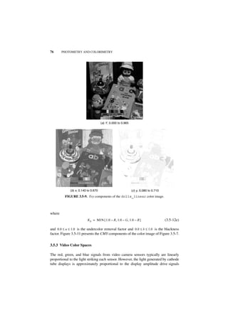
Figure 6.3-1 contains photographs of an image linearly quantized with a variable
number of quantization levels. The source image is a split image in which the left
side is a luminance image and the right side is a computer-generated linear ramp. In
Figure 6.3-1, the luminance signal of the image has been uniformly quantized with
from 8 to 256 levels (3 to 8 bits). Gray scale contouring in these pictures is apparent
in the ramp part of the split image for 6 or fewer bits. The contouring of the lumi-
nance image part of the split image becomes noticeable for 5 bits.
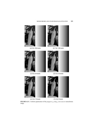
As discussed in Section 2-4, it has been postulated that the eye responds
logarithmically or to a power law of incident light amplitude. There have been several
efforts to quantitatively model this nonlinear response by a lightness function Λ ,
which is related to incident luminance. Priest et al. (9) have proposed a square-root
nonlinearity
1⁄2
Λ = ( 100.0Y ) (6.3-2)
where 0.0 ≤ Y ≤ 1.0 and 0.0 ≤ Λ ≤ 10.0 . Ladd and Pinney (10) have suggested a cube-
root scale
1⁄3
Λ = 2.468 ( 100.0Y ) – 1.636 (6.3-3)
A logarithm scale
Λ = 5.0 [ log { 100.0Y } ] (6.3-4)
10](https://image.slidesharecdn.com/digitalimageprocessing-120319064358-phpapp01/85/Digital-image-processing-163-320.jpg)


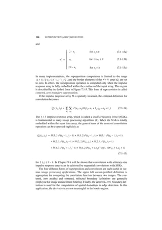
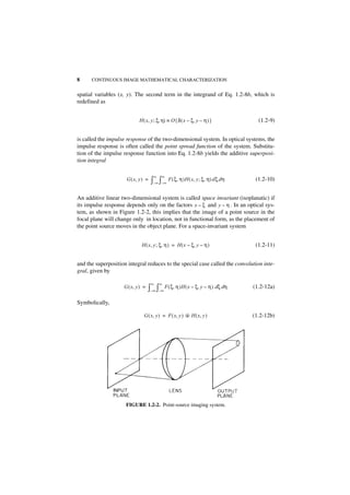
![172 SUPERPOSITION AND CONVOLUTION
˜
where W ( k 1 , k 2 ) is a weighting coefficient for the particular quadrature formula
employed. Usually, a rectangular quadrature formula is used, and the weighting
coefficients are unity. In any case, it is notationally convenient to lump the weight-
ing coefficient and the impulse response function together so that
˜ ˜ ˜
H ( j1 ∆S, j 2 ∆S; k 1 ∆I, k 2 ∆I) = W ( k 1, k 2 )J ( j 1 ∆S, j 2 ∆S ; k 1 ∆I, k 2 ∆I) (7.2-8)
Then,
K 1U K 2U
˜ ˜ ˜
G ( j 1 ∆S, j 2 ∆S) = ∑ ∑ F ( k 1 ∆I, k 2 ∆I )H ( j 1 ∆S, j 2 ∆S ; k 1 ∆I, k 2 ∆I ) (7.2-9)
k 1 = K 1L k 2 = K 2L
˜
Again, it should be noted that H is not spatially discretized; the function is simply
evaluated at its appropriate spatial argument. The limits of summation of Eq. 7.2-9
are
∆S T ∆S T
K iL = j i ------ – -----
- - K iU = ji ------ + -----
- - (7.2-10)
∆I ∆I N ∆I ∆I N
where [ · ] N denotes the nearest integer value of the argument.
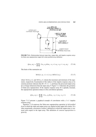
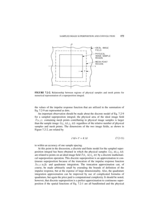
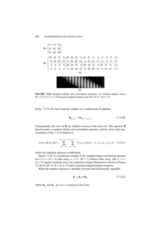
Figure 7.2-1 provides an example relating actual physical sample values
˜ ˜
G ( j1 ∆ S, j2 ∆S) to mesh points F ( k 1 ∆I, k 2 ∆I ) on the ideal image field. In this exam-
ple, the mesh spacing is twice as large as the physical sample spacing. In the figure,
FIGURE 7.2-1. Relationship of physical image samples to mesh points on an ideal image
field for numerical representation of a superposition integral.](https://image.slidesharecdn.com/digitalimageprocessing-120319064358-phpapp01/85/Digital-image-processing-182-320.jpg)
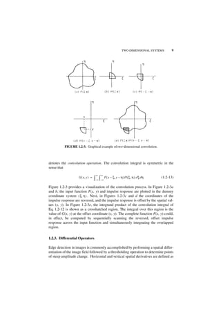
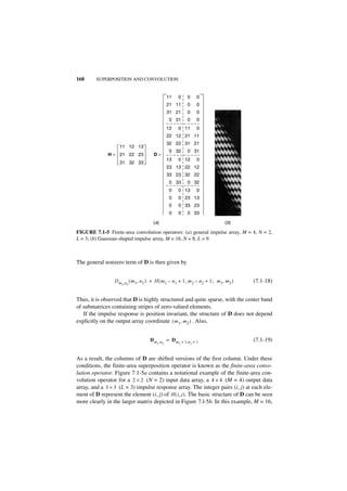
![SAMPLED IMAGE SUPERPOSITION AND CONVOLUTION 175
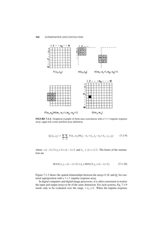
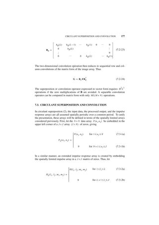
FIGURE 7.2-3. Sampled image arrays.
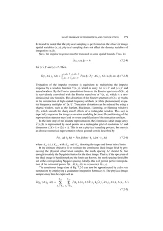
The general term of B is defined as
Bm
2, n 2 ( m 1, n 1 ) = H ( m1 ∆S, m 2 ∆S ; n 1 ∆I, n 2 ∆I ) (7.2-16)
for 1 ≤ m i ≤ M and m i ≤ n i ≤ m i + L – 1 where L = [ 2T ⁄ ∆I ] N represents the nearest
odd integer dimension of the impulse response in resolution units ∆I . For descrip-
tional simplicity, B is called the blur matrix of the superposition integral.
If the impulse response function is translation invariant such that
H ( m 1 ∆S, m 2 ∆S ; n 1 ∆I, n 2 ∆I ) = H ( m 1 ∆S – n 1 ∆I, m2 ∆S – n 2 ∆I ) (7.2-17)
then the discrete superposition operation of Eq. 7.2-13 becomes a discrete convolu-
tion operation of the form
N 1U N 2U
G ( m 1 ∆S, m 2 ∆S ) = ∑ ∑ F ( n 1 ∆I, n 2 ∆I )H ( m1 ∆S – n 1 ∆I, m 2 ∆S – n 2 ∆I )
n 1 = N 1L n 2 = N 2L
(7.2-18)
If the physical sample and quadrature mesh spacings are equal, the general term
of the blur matrix assumes the form
Bm
2, n 2 ( m 1, n 1 ) = H ( m 1 – n 1 + L, m 2 – n 2 + L ) (7.2-19)](https://image.slidesharecdn.com/digitalimageprocessing-120319064358-phpapp01/85/Digital-image-processing-185-320.jpg)
![SUPERPOSITION AND CONVOLUTION OPERATOR RELATIONSHIPS 181
(K)
S1 J = IK 0 (7.4-1a)
(K )
S2 J = 0A IK 0 (7.4-1b)
(K) (K)
where S1 J and S2 J are K × J matrices, IK is a K × K identity matrix, and 0 A is a
K × L – 1 matrix. For future reference, it should be noted that the generalized
inverses of S1 and S2 and their transposes are
(K) – ( K) T
[ S1 J ] = [ S1 J ] (7.4-2a)
( K) T – K
[ [ S1 J ] ] = S1 J (7.4-2b)
( K) – (K) T
[ S2 J ] = [ S2 J ] (7.4-2c)
( K) T – K
[ [ S2 J ] ] = S2 J (7.4-2d)
Examination of the structure of the various superposition operators indicates that
(M) (M) ( N) (N) T
D = [ S1 J ⊗ S1 J ]C [ S1 J ⊗ S1 J ] (7.4-3a)
(M) (M) ( N) ( N) T
B = [ S2 J ⊗ S2 J ]C [ S1 J ⊗ S1 J ] (7.4-3b)
That is, the matrix D is obtained by extracting the first M rows and N columns of sub-
matrices Cmn of C. The first M rows and N columns of each submatrix are also
extracted. A similar explanation holds for the extraction of B from C. In Figure 7.3-1,
the elements of C to be extracted to form D and B are indicated by boxes.
From the definition of the extended input data array of Eq. 7.3-1, it is obvious
that the spatially limited input data vector f can be obtained from the extended data
vector fE by the selection operation
(N) (N )
f = [ S1 J ⊗ S1 J ]f E (7.4-4a)
and furthermore,
( N) ( N) T
fE = [ S1 J ⊗ S1 J ] f (7.4-4b)](https://image.slidesharecdn.com/digitalimageprocessing-120319064358-phpapp01/85/Digital-image-processing-191-320.jpg)
![182 SUPERPOSITION AND CONVOLUTION
It can also be shown that the output vector for finite-area superposition can be
obtained from the output vector for circulant superposition by the selection opera-
tion
(M) (M)
q = [ S1 J ⊗ S1 J ]k E (7.4-5a)
The inverse relationship also exists in the form
(M) (M) T
k E = [ S1J ⊗ S1 J ] q (7.4-5b)
For sampled image superposition
(M) (M)
g = [ S2 J ⊗ S2 J ]k E (7.4-6)
but it is not possible to obtain kE from g because of the underdeterminacy of the
sampled image superposition operator. Expressing both q and kE of Eq. 7.4-5a in
matrix form leads to
M J
(M) (M)
∑ ∑ Mm [ S1J
T T
Q = ⊗ S1 J ]N n K E v n u m (7.4-7)
m=1 n=1
As a result of the separability of the selection operator, Eq. 7.4-7 reduces to
(M) (M) T
Q = [ S1 J ]K E [ S1 J ] (7.4-8)
Similarly, for Eq. 7.4-6 describing sampled infinite-area superposition,
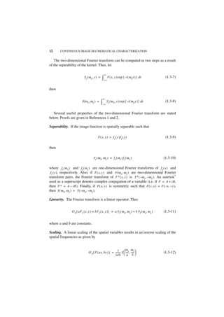
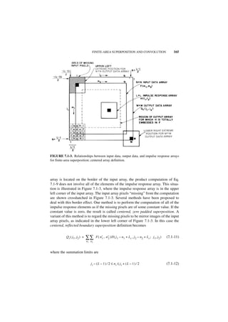
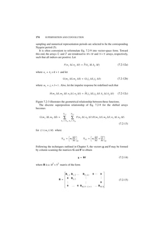
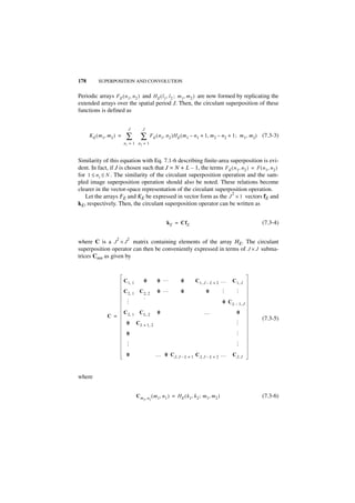
FIGURE 7.4-1. Location of elements of processed data Q and G from KE.](https://image.slidesharecdn.com/digitalimageprocessing-120319064358-phpapp01/85/Digital-image-processing-192-320.jpg)
![REFERENCES 183
(M) (M) T
G = [ S2 J ]K E [ S2 J ] (7.4-9)
Figure 7.4-1 illustrates the locations of the elements of G and Q extracted from KE
for finite-area and sampled infinite-area superposition.
In summary, it has been shown that the output data vectors for either finite-area
or sampled image superposition can be obtained by a simple selection operation on
the output data vector of circulant superposition. Computational advantages that can
be realized from this result are considered in Chapter 9.
REFERENCES
1. J. F. Abramatic and O. D. Faugeras, “Design of Two-Dimensional FIR Filters from
Small Generating Kernels,” Proc. IEEE Conference on Pattern Recognition and Image
Processing, Chicago, May 1978.
2. W. K. Pratt, “Vector Formulation of Two Dimensional Signal Processing Operations,”
Computer Graphics and Image Processing, 4, 1, March 1975, 1–24.
3. A. V. Oppenheim and R. W. Schaefer (Contributor), Digital Signal Processing, Prentice
Hall, Englewood Cliffs, NJ, 1975.
4. T. R. McCalla, Introduction to Numerical Methods and FORTRAN Programming, Wiley,
New York, 1967.
5. A. Papoulis, Systems and Transforms with Applications in Optics, 2nd ed., McGraw-
Hill, New York, 1981.](https://image.slidesharecdn.com/digitalimageprocessing-120319064358-phpapp01/85/Digital-image-processing-193-320.jpg)

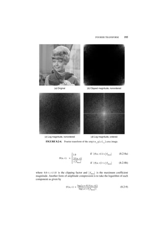
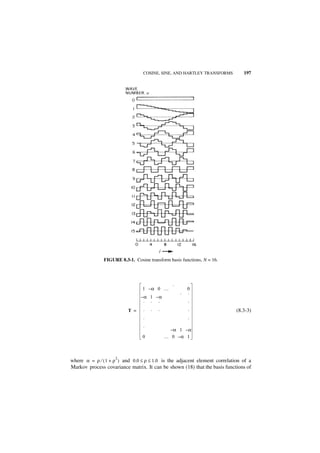
![196 UNITARY TRANSFORMS
8.3.1. Cosine Transform
The cosine transform, discovered by Ahmed et al. (12), has found wide application
in transform image coding. In fact, it is the foundation of the JPEG standard (13) for
still image coding and the MPEG standard for the coding of moving images (14).
The forward cosine transform is defined as (12)
N–1 N–1
2 π 1 π 1
F ( u, v ) = --- C ( u )C ( v )
N
- ∑ ∑ F ( j, k ) cos --- [ u ( j + --- ) ] cos --- [ v ( k + --- ) ]
N
-
2
N
-
2
j=0 k=0
(8.3-1a)
N–1 N–1
2 π 1 π 1
F ( j, k ) = ---
N
- ∑ ∑ C ( u )C ( v )F ( u, v ) cos --- [ u ( j + --- ) ] cos --- [ v ( k + --- ) ]
N
-
2
N
-
2
j=0 k=0
(8.3-1b)
–1 ⁄ 2
where C ( 0 ) = ( 2 ) and C ( w ) = 1 for w = 1, 2,..., N – 1. It has been observed
that the basis functions of the cosine transform are actually a class of discrete Che-
byshev polynomials (12).
Figure 8.3-1 is a plot of the cosine transform basis functions for N = 16. A photo-
graph of the cosine transform of the test image of Figure 8.2-4a is shown in Figure
8.3-2a. The origin is placed in the upper left corner of the picture, consistent with
matrix notation. It should be observed that as with the Fourier transform, the image
energy tends to concentrate toward the lower spatial frequencies.
The cosine transform of a N × N image can be computed by reflecting the image
about its edges to obtain a 2N × 2N array, taking the FFT of the array and then
extracting the real parts of the Fourier transform (15). Algorithms also exist for the
direct computation of each row or column of Eq. 8.3-1 with on the order of N log N
real arithmetic operations (12,16).
8.3.2. Sine Transform
The sine transform, introduced by Jain (17), as a fast algorithmic substitute for the
Karhunen–Loeve transform of a Markov process is defined in one-dimensional form
by the basis functions
2 ( j + 1 ) ( u + 1 )π
A ( u, j ) = ------------ sin -------------------------------------
- - (8.3-2)
N+1 N+1
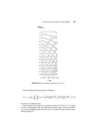
for u, j = 0, 1, 2,..., N – 1. Consider the tridiagonal matrix](https://image.slidesharecdn.com/digitalimageprocessing-120319064358-phpapp01/85/Digital-image-processing-205-320.jpg)

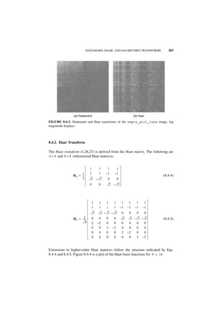
![HADAMARD, HAAR, AND DAUBECHIES TRANSFORMS 205
1 –1 0 0 0 0 … 0 0 0 0
0 0 1 –1 0 0 … 0 0 0 0
1
W N = ------
- (8.4-7b)
…
…
2
0 0 0 0 0 0 … 1 –1 0 0
0 0 0 0 0 0 … 0 0 1 –1
The elements of the rows of V N are called first-level scaling signals, and the
elements of the rows of W N are called first-level Haar wavelets (29).
The first-level Haar transform of a N × 1 vector f is
T
f1 = R N f = [ a 1 d1 ] (8.4-8)
where
a1 = VN f (8.4-9a)
d 1 = WN f (8.4-9b)
The vector a 1 represents the running average or trend of the elements of f , and the
vector d1 represents the running fluctuation of the elements of f . The next step in
the recursion process is to compute the second-level Haar transform from the trend
part of the first-level transform and concatenate it with the first-level fluctuation
vector. This results in
T
f 2 = [ a2 d2 d1 ] (8.4-10)
where
a 2 = VN ⁄ 2 a1 (8.4-11a)
d2 = WN ⁄ 2 a 1 (8.4-11b)
are N ⁄ 4 × 1 vectors. The process continues until the full transform
T
f ≡ fn = [ an d n d n – 1 … d 1 ] (8.4-12)
n
is obtained where N = 2 . It should be noted that the intermediate levels are unitary
transforms.](https://image.slidesharecdn.com/digitalimageprocessing-120319064358-phpapp01/85/Digital-image-processing-214-320.jpg)

![KARHUNEN–LOEVE TRANSFORM 207
In Eqs. 8.4-13a and 8.4-13b, the row-to-row shift is by two elements, and the last
two scale factors wrap around on the last rows. Following the recursion process of
the Haar transform results in the Daub4 transform final stage:
T
f ≡ f n = [ an dn dn – 1 … d 1 ] (8.4-15)
Daubechies has extended the wavelet transform concept for higher degrees of
support, 6, 8, 10,..., by straightforward extension of Eq. 8.4-13 (29). Daubechies
also has also constructed another family of wavelets, called coiflets, after a sugges-
tion of Coifman (29).
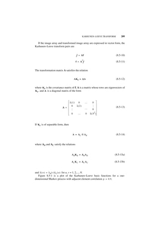
8.5. KARHUNEN–LOEVE TRANSFORM
Techniques for transforming continuous signals into a set of uncorrelated represen-
tational coefficients were originally developed by Karhunen (31) and Loeve (32).
Hotelling (33) has been credited (34) with the conversion procedure that transforms
discrete signals into a sequence of uncorrelated coefficients. However, most of the
literature in the field refers to both discrete and continuous transformations as either
a Karhunen–Loeve transform or an eigenvector transform.
The Karhunen–Loeve transformation is a transformation of the general form
N–1 N–1
F ( u, v ) = ∑ ∑ F ( j, k )A ( j, k ; u, v ) (8.5-1)
j=0 k=0
for which the kernel A(j, k; u, v) satisfies the equation
N–1 N–1
λ ( u, v )A ( j, k ; u, v ) = ∑ ∑ K F ( j, k ; j′, k′ ) A ( j′, k′ ; u, v ) (8.5-2)
j′ = 0 k′ = 0
where KF ( j, k ; j′, k′ ) denotes the covariance function of the image array and λ ( u, v )
is a constant for fixed (u, v). The set of functions defined by the kernel are the eigen-
functions of the covariance function, and λ ( u, v ) represents the eigenvalues of the
covariance function. It is usually not possible to express the kernel in explicit form.
If the covariance function is separable such that
K F ( j, k ; j′, k′ ) = K C ( j, j′ )K R ( k, k′ ) (8.5-3)
then the Karhunen-Loeve kernel is also separable and
A ( j, k ; u , v ) = A C ( u, j )AR ( v, k ) (8.5-4)](https://image.slidesharecdn.com/digitalimageprocessing-120319064358-phpapp01/85/Digital-image-processing-216-320.jpg)
![208 UNITARY TRANSFORMS
The row and column kernels satisfy the equations
N–1
λ R ( u )AR ( v, k ) = ∑ K R ( k, k′ )A R ( v, k′ ) (8.5-5a)
k′ = 0
N–1
λ C ( v )A C ( u, j ) = ∑ KC ( j, j′ )AC ( u, j′ ) (8.5-5b)
j′ = 0
In the special case in which the covariance matrix is of separable first-order Markov
process form, the eigenfunctions can be written in explicit form. For a one-dimen-
sional Markov process with correlation factor ρ , the eigenfunctions and eigenvalues
are given by (35)
2 1⁄2 N–1 ( u + 1 )π
A ( u, j ) = -----------------------
- sin w ( u ) j – ------------ + --------------------
- (8.5-6)
2
N + λ ( u) 2 2
and
2
1–ρ
λ ( u ) = --------------------------------------------------------
- for 0 ≤ j, u ≤ N – 1 (8.5-7)
2
1 – 2ρ cos { w ( u ) } + ρ
where w(u) denotes the root of the transcendental equation
2
( 1 – ρ ) sin w
tan { Nw } = --------------------------------------------------
- (8.5-8)
2
cos w – 2ρ + ρ cos w
The eigenvectors can also be generated by the recursion formula (36)
λ(u)
A ( u, 0 ) = -------------- [ A ( u, 0 ) – ρA ( u, 1 ) ] (8.5-9a)
2
1–ρ
λ(u) 2
A ( u, j ) = -------------- [ – ρA ( u, j – 1 ) + ( 1 + ρ )A ( u, j ) – ρA ( u, j + 1 ) ] for 0 < j < N – 1
2
1–ρ
(8.5-9b)
λ( u)
A ( u, N – 1 ) = -------------- [ – ρA ( u, N – 2 ) + ρA ( u, N – 1 ) ] (8.5-9c)
2
1–ρ
by initially setting A(u, 0) = 1 and subsequently normalizing the eigenvectors.](https://image.slidesharecdn.com/digitalimageprocessing-120319064358-phpapp01/85/Digital-image-processing-217-320.jpg)


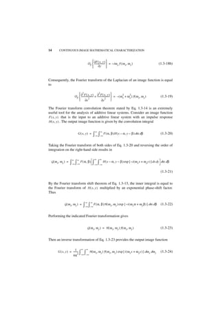
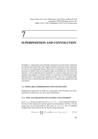
![214 LINEAR PROCESSING TECHNIQUES
FIGURE 9.1-1. Direct processing and generalized linear filtering; series formulation.
Figure 9.1-1 is a block diagram of the indirect computation technique called gen-
eralized linear filtering (1). In the process, the input array F ( n1, n 2 ) undergoes a
two-dimensional unitary transformation, resulting in an array of transform coeffi-
cients F ( u 1, u 2 ) . Next, a linear combination of these coefficients is taken according
to the general relation
M1 M2
˜
F ( w 1, w 2 ) = ∑ ∑ F ( u 1, u 2 )T ( u 1, u 2 ; w 1, w 2 ) (9.1-3)
u1 = 1 u2 = 1
where T ( u 1, u 2 ; w 1, w 2 ) represents the linear filtering transformation function.
Finally, an inverse unitary transformation is performed to reconstruct the processed
array P ( m1, m 2 ) . If this computational procedure is to be more efficient than direct
computation by Eq. 9.1-1, it is necessary that fast computational algorithms exist for
the unitary transformation, and also the kernel T ( u 1, u 2 ; w 1, w 2 ) must be reasonably
sparse; that is, it must contain many zero elements.
The generalized linear filtering process can also be defined in terms of vector-
space computations as shown in Figure 9.1-2. For notational simplicity, let N1 = N2
= N and M1 = M2 = M. Then the generalized linear filtering process can be described
by the equations
f = [ A 2 ]f (9.1-4a)
N
˜ = Tf
f f (9.1-4b)
] ˜
–1
p = [A 2 f (9.1-4c)
M](https://image.slidesharecdn.com/digitalimageprocessing-120319064358-phpapp01/85/Digital-image-processing-223-320.jpg)
![TRANSFORM DOMAIN PROCESSING 215
FIGURE 9.1-2. Direct processing and generalized linear filtering; vector formulation.
2 2 2 2
where A 2 is a N × N unitary transform matrix, T is a M × N linear filtering
N 2 2
transform operation, and A 2 is a M × M unitary transform matrix. From
M
Eq. 9.1-4, the input and output vectors are related by
–1
p = [A 2 ] T [ A 2 ]f (9.1-5)
M N
Therefore, equating Eqs. 9.1-2 and 9.1-5 yields the relations between T and T given
by
–1
T = [A 2 ] T [A 2] (9.1-6a)
M N
–1
T = [A 2 ]T [ A 2 ] (9.1-6b)
M N
2 2
If direct processing is employed, computation by Eq. 9.1-2 requires k P ( M N ) oper-
ations, where 0 ≤ k P ≤ 1 is a measure of the sparseness of T. With the generalized
linear filtering technique, the number of operations required for a given operator are:
4
Forward transform: N by direct transformation
2
2N log 2 N by fast transformation
2 2
Filter multiplication: kT M N
4
Inverse transform: M by direct transformation
2
2M log 2 M by fast transformation](https://image.slidesharecdn.com/digitalimageprocessing-120319064358-phpapp01/85/Digital-image-processing-224-320.jpg)
![216 LINEAR PROCESSING TECHNIQUES
where 0 ≤ k T ≤ 1 is a measure of the sparseness of T. If k T = 1 and direct unitary
transform computation is performed, it is obvious that the generalized linear filter-
ing concept is not as efficient as direct computation. However, if fast transform
algorithms, similar in structure to the fast Fourier transform, are employed, general-
ized linear filtering will be more efficient than direct processing if the sparseness
index satisfies the inequality
2 2
k T < k P – ------ log 2 N – ----- log 2 M
- - (9.1-7)
2 2
M N
In many applications, T will be sufficiently sparse such that the inequality will be
satisfied. In fact, unitary transformation tends to decorrelate the elements of T caus-
ing T to be sparse. Also, it is often possible to render the filter matrix sparse by
setting small-magnitude elements to zero without seriously affecting computational
accuracy (1).
In subsequent sections, the structure of superposition and convolution operators
is analyzed to determine the feasibility of generalized linear filtering in these appli-
cations.
9.2. TRANSFORM DOMAIN SUPERPOSITION
The superposition operations discussed in Chapter 7 can often be performed more
efficiently by transform domain processing rather than by direct processing. Figure
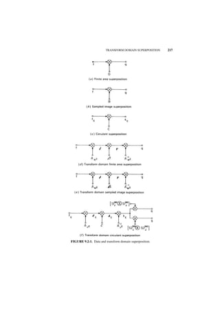
9.2-1a and b illustrate block diagrams of the computational steps involved in direct
finite area or sampled image superposition. In Figure 9.2-1d and e, an alternative
form of processing is illustrated in which a unitary transformation operation is per-
formed on the data vector f before multiplication by a finite area filter matrix D or
sampled image filter matrix B. An inverse transform reconstructs the output vector.
From Figure 9.2-1, for finite-area superposition, because
q = Df (9.2-1a)
and
–1
q = [A 2 ] D [ A 2 ]f (9.2-1b)
M N
then clearly the finite-area filter matrix may be expressed as
–1
D = [A 2 ]D [ A 2 ] (9.2-2a)
M N](https://image.slidesharecdn.com/digitalimageprocessing-120319064358-phpapp01/85/Digital-image-processing-225-320.jpg)
![218 LINEAR PROCESSING TECHNIQUES
Similarly,
–1
B = [A 2 ]B [ A 2 ] (9.2-2b)
M N
If direct finite-area superposition is performed, the required number of
2 2
computational operations is approximately N L , where L is the dimension of the
impulse response matrix. In this case, the sparseness index of D is
L 2
k D = ---
N - (9.2-3a)
2 2
Direct sampled image superposition requires on the order of M L operations, and
the corresponding sparseness index of B is
L 2
k B = ----
- (9.2-3b)
M
Figure 9.2-1f is a block diagram of a system for performing circulant superposition
by transform domain processing. In this case, the input vector kE is the extended
data vector, obtained by embedding the input image array F ( n1, n 2 ) in the left cor-
ner of a J × J array of zeros and then column scanning the resultant matrix. Follow-
ing the same reasoning as above, it is seen that
–1
k E = Cf E = [ A 2 ] C [ A 2 ]f (9.2-4a)
J J
and hence,
–1
C = [ A 2 ]C [ A 2 ] (9.2-4b)
J J
As noted in Chapter 7, the equivalent output vector for either finite-area or sampled
image superposition can be obtained by an element selection operation of kE. For
finite-area superposition,
(M) (M)
q = [ S1 J ⊗ S1 J ]k E (9.2-5a)
and for sampled image superposition
(M) (M)
g = [ S2 J ⊗ S2 J ]k E (9.2-5b)](https://image.slidesharecdn.com/digitalimageprocessing-120319064358-phpapp01/85/Digital-image-processing-227-320.jpg)
![TRANSFORM DOMAIN SUPERPOSITION 219
Also, the matrix form of the output for finite-area superposition is related to the
extended image matrix KE by
(M) (M) T
Q = [ S1 J ]K E [ S1 J ] (9.2-6a)
For sampled image superposition,
(M) (M) T
G = [ S2 J ]K E [ S2 J ] (9.2-6b)
The number of computational operations required to obtain kE by transform domain
processing is given by the previous analysis for M = N = J.
4
Direct transformation 3J
2 2
Fast transformation: J + 4J log 2 J
2
If C is sparse, many of the J filter multiplication operations can be avoided.
From the discussion above, it can be seen that the secret to computationally effi-
cient superposition is to select a transformation that possesses a fast computational
algorithm that results in a relatively sparse transform domain superposition filter
matrix. As an example, consider finite-area convolution performed by Fourier
domain processing (2,3). Referring to Figure 9.2-1, let
A 2 = AK ⊗ AK (9.2-7)
K
where
1 - ( x – 1) (y – 1 )
AK = ------- W with W ≡ exp – 2πi
-----------
K K
(K) 2
for x, y = 1, 2,..., K. Also, let h E denote the K × 1 vector representation of the
extended spatially invariant impulse response array of Eq. 7.3-2 for J = K. The Fou-
(K)
rier transform of h E is denoted as
(K) (K )
hE = [ A 2 ]h E (9.2-8)
K
2 2
These transform components are then inserted as the diagonal elements of a K × K
matrix
( K) ( K) (K) 2
H = diag [ h E ( 1 ), …, h E ( K ) ] (9.2-9)](https://image.slidesharecdn.com/digitalimageprocessing-120319064358-phpapp01/85/Digital-image-processing-228-320.jpg)
![220 LINEAR PROCESSING TECHNIQUES
Then, it can be shown, after considerable manipulation, that the Fourier transform
domain superposition matrices for finite area and sampled image convolution can be
written as (4)
(M)
D = H [ PD ⊗ PD ] (9.2-10)
for N = M – L + 1 and
(N)
B = [ PB ⊗ PB ] H (9.2-11)
where N = M + L + 1 and
–(u – 1 ) (L – 1 )
1 1 – WM
P D ( u, v ) = -------- ---------------------------------------------------------------
- - (9.2-12a)
M 1 – W M – ( u – 1 ) – W N –( v – 1 )
–( v – 1 ) ( L – 1 )
1 1 – WN
PB ( u, v ) = ------- ---------------------------------------------------------------
- - (9.2-12b)
N 1 – W M –( u – 1 ) – W N– ( v – 1 )
Thus the transform domain convolution operators each consist of a scalar weighting
(K )
matrix H and an interpolation matrix ( P ⊗ P ) that performs the dimensionality con-
2 2
version between the N - element input vector and the M - element output vector.
Generally, the interpolation matrix is relatively sparse, and therefore, transform domain
superposition is quite efficient.
Now, consider circulant area convolution in the transform domain. Following the
previous analysis it is found (4) that the circulant area convolution filter matrix
reduces to a scalar operator
(J )
C = JH (9.2-13)
Thus, as indicated in Eqs. 9.2-10 to 9.2-13, the Fourier domain convolution filter
matrices can be expressed in a compact closed form for analysis or operational stor-
age. No closed-form expressions have been found for other unitary transforms.
Fourier domain convolution is computationally efficient because the convolution
operator C is a circulant matrix, and the corresponding filter matrix C is of diagonal
form. Actually, as can be seen from Eq. 9.1-6, the Fourier transform basis vectors
are eigenvectors of C (5). This result does not hold true for superposition in general,
nor for convolution using other unitary transforms. However, in many instances, the
filter matrices D, B, and C are relatively sparse, and computational savings can
often be achieved by transform domain processing.](https://image.slidesharecdn.com/digitalimageprocessing-120319064358-phpapp01/85/Digital-image-processing-229-320.jpg)
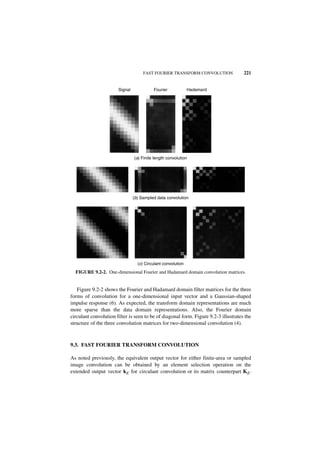
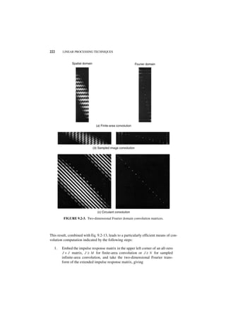
![FAST FOURIER TRANSFORM CONVOLUTION 223
HE = AJ HE AJ (9.3-1)
2. Embed the input data array in the upper left corner of an all-zero J × J
matrix, and take the two-dimensional Fourier transform of the extended
input data matrix to obtain
FE = A J FE A J (9.3-2)
3. Perform the scalar multiplication
K E ( m, n ) = JH E ( m, n )F E ( m, n ) (9.3-3)
where 1 ≤ m, n ≤ J .
4. Take the inverse Fourier transform
–1 –1
KE = [ A 2 ] HE [ A 2 ] (9.3-4)
J J
5. Extract the desired output matrix
(M) (M) T
Q = [ S1 J ]K E [ S1 J ] (9.3-5a)
or
(M) (M) T
G = [ S2 J ]K E [ S2 J ] (9.3-5b)
It is important that the size of the extended arrays in steps 1 and 2 be chosen large
enough to satisfy the inequalities indicated. If the computational steps are performed
with J = N, the resulting output array, shown in Figure 9.3-1, will contain erroneous
terms in a boundary region of width L – 1 elements, on the top and left-hand side of
the output field. This is the wraparound error associated with incorrect use of the
Fourier domain convolution method. In addition, for finite area (D-type) convolu-
tion, the bottom and right-hand-side strip of output elements will be missing. If the
computation is performed with J = M, the output array will be completely filled with
the correct terms for D-type convolution. To force J = M for B-type convolution, it is
necessary to truncate the bottom and right-hand side of the input array. As a conse-
quence, the top and left-hand-side elements of the output array are erroneous.](https://image.slidesharecdn.com/digitalimageprocessing-120319064358-phpapp01/85/Digital-image-processing-232-320.jpg)
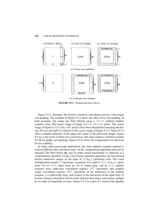
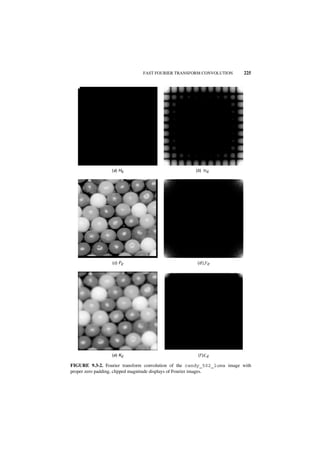
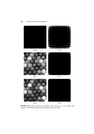

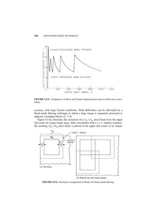
![230 LINEAR PROCESSING TECHNIQUES
∞
gC ( x ) = ∫–∞ fC ( α )hC ( x – α ) dα (9.4-1a)
or in the continuous Fourier domain by
1 ∞
g C ( x ) = -----
2π
- ∫–∞ fC ( ω )hC ( ω ) exp { iωx } dω (9.4-1b)
Chapter 7 has presented techniques for the discretization of the convolution inte-
gral of Eq. 9.4-1. In this process, the continuous impulse response function h C ( x )
must be truncated by spatial multiplication of a window function y(x) to produce the
windowed impulse response
b C ( x ) = h C ( x )y ( x ) (9.4-2)
where y(x) = 0 for x > T . The window function is designed to smooth the truncation
effect. The resulting convolution integral is then approximated as
x+T
gC ( x ) = ∫x – T fC ( α )b C ( x – α ) dα (9.4-3)
Next, the output signal g C ( x ) is sampled over 2J + 1 points at a resolution
∆ = π ⁄ ω 0, and the continuous integration is replaced by a quadrature summation at
the same resolution ∆ , yielding the discrete representation
j+K
g C ( j∆ ) = ∑ f C ( k∆ )b C [ ( j – k )∆ ] (9.4-4)
k=j–K
where K is the nearest integer value of the ratio T ⁄ ∆.
Computation of Eq. 9.4-4 by discrete Fourier transform processing requires
formation of the discrete domain transfer function b D ( u ) . If the continuous domain
impulse response function h C ( x ) is known analytically, the samples of the
windowed impulse response function are inserted as the first L = 2K + 1 elements of
a J-element sequence and the remaining J – L elements are set to zero. Thus, let
b D ( p ) = b C ( – K ), …, b C ( 0 ), …, b C ( K ) , 0, …, 0 (9.4-5)
L terms
where 0 ≤ p ≤ P – 1. The terms of b D ( p ) can be extracted from the continuous
impulse response function h C ( x ) and the window function by the sampling
operation](https://image.slidesharecdn.com/digitalimageprocessing-120319064358-phpapp01/85/Digital-image-processing-239-320.jpg)
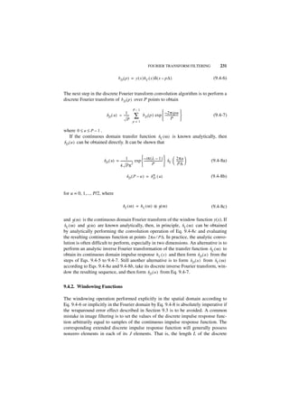
![232 LINEAR PROCESSING TECHNIQUES
impulse response embedded in the extended vector of Eq. 9.4-5 will implicitly be set
equal to J. Therefore, all elements of the output filtering operation will be subject to
wraparound error.
A variety of window functions have been proposed for discrete linear filtering
(10–12). Several of the most common are listed in Table 9.4-1 and sketched in
Figure 9.4-1. Figure 9.4-2 shows plots of the transfer functions of these window
functions. The window transfer functions consist of a main lobe and sidelobes
whose peaks decrease in magnitude with increasing frequency. Examination of the
structure of Eq. 9.4-8 indicates that the main lobe causes a loss in frequency
response over the signal passband from 0 to ω 0 , while the sidelobes are responsible
for an aliasing error because the windowed impulse response function b C ( ω ) is not
bandlimited. A tapered window function reduces the magnitude of the sidelobes and
consequently attenuates the aliasing error, but the main lobe becomes wider, causing
the signal frequency response within the passband to be reduced. A design trade-off
must be made between these complementary sources of error. Both sources of
degradation can be reduced by increasing the truncation length of the windowed
impulse response, but this strategy will either result in a shorter length output
sequence or an increased number of computational operations.
TABLE 9.4-1. Window Functions a
Function Definition
Rectangular w(n) = 1 0≤n≤L–1
2n -
----------- 0≤n–L–1
-----------
-
L–1 2
Barlett (triangular) w(n) =
2
2 – ----------- L–1
- ----------- ≤ n ≤ L – 1
-
L–1 2
1 2πn
Hanning w(n) = -- 1 – cos -----------
- - 0≤n≤L–1
2 L – 1
2πn-
Hamming w(n) = 0.54 - 0.46 cos ----------- 0≤n≤L–1
L – 1
2πn 4πn
Blackman w(n) = 0.42 – 0.5 cos ----------- + 0.08 cos -----------
- - 0≤n≤L–1
L–1 L – 1
2 2 1 ⁄ 2
I0 ωa [ ( ( L – 1 ) ⁄ 2 ) – [ n – ( ( L – 1 ) ⁄ 2 ) ] ]
Kaiser
----------------------------------------------------------------------------------------------------------------- 0 ≤ n ≤ L – 1
-
I0 { ωa [ ( L – 1 ) ⁄ 2 ] }
a
I 0 { · } is the modified zeroth-order Bessel function of the first kind and ω a is a design parameter.](https://image.slidesharecdn.com/digitalimageprocessing-120319064358-phpapp01/85/Digital-image-processing-241-320.jpg)
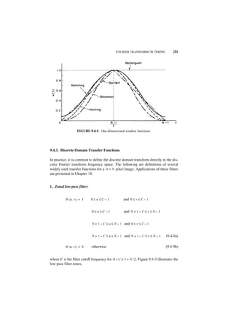
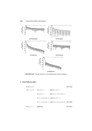
![FOURIER TRANSFORM FILTERING 235
FIGURE 9.4-3. Zonal filter transfer function definition.
3. Gaussian filter:
H ( u, v ) = G ( u, v ) 0≤u≤N⁄2 and 0 ≤ v ≤ N ⁄ 2
0≤u≤N⁄2 and 1 + N ⁄ 2 ≤ v ≤ N – 1
1 + N ⁄ 2 ≤ u ≤ N – 1 and 0 ≤ v ≤ N ⁄ 2
1 + N ⁄ 2 ≤ u ≤ N – 1 and 1 + N ⁄ 2 ≤ v ≤ N – 1 (9.4-11a)
where
1 2 2
G ( u, v ) = exp – -- [ ( s u u ) + ( s v v ) ]
- (9.4-11b)
2
and su and sv are the Gaussian filter spread factors.](https://image.slidesharecdn.com/digitalimageprocessing-120319064358-phpapp01/85/Digital-image-processing-244-320.jpg)
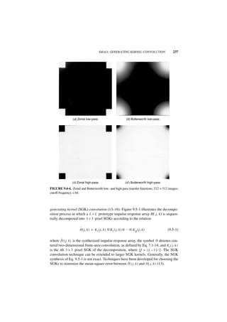
![238 LINEAR PROCESSING TECHNIQUES
FIGURE 9.5-1. Cascade decomposition of a two-dimensional impulse response array into
small generating kernels.
Two-dimensional convolution can be performed sequentially without approxima-
tion error by utilizing the singular-value decomposition technique described in
Appendix A1.2 in conjunction with the SGK decimation (17–19). With this method,
called SVD/SGK convolution, the impulse response array H ( j, k ) is regarded as a
matrix H. Suppose that H is orthogonally separable such that it can be expressed in
the outer product form
T
H = ab (9.5-2)
where a and b are column and row operator vectors, respectively. Then, the two-
dimensional convolution operation can be performed by first convolving the col-
umns of F ( j, k ) with the impulse response sequence a(j) corresponding to the vec-
tor a, and then convolving the rows of that resulting array with the sequence b(k)
corresponding to the vector b. If H is not separable, the matrix can be expressed as a
sum of separable matrices by the singular-value decomposition by which
R
H = ∑ Hi (9.5-3a)
i=1
T
Hi = si ai bi (9.5-3b)
where R ≥ 1 is the rank of H, si is the ith singular value of H. The vectors ai and bi
are the L × 1 eigenvectors of HHT and HTH, respectively.
Each eigenvector ai and bi of Eq. 9.5-3 can be considered to be a one-dimen-
sional sequence, which can be decimated by a small generating kernel expansion as
a i ( j ) = c i [ a i1 ( j ) ᭺ … ᭺ a iq ( j ) ᭺ … ᭺ a iQ ( j ) ]
ء ء ء ء (9.5-4a)
b i ( k ) = r i [ b i1 ( k ) ᭺ … ᭺ b iq ( k ) ᭺ … ᭺ b iQ ( k ) ]
ء ء ء ء (9.5-4b)
where a iq ( j ) and b iq ( k ) are 3 × 1 impulse response sequences corresponding to the
ith singular-value channel and the qth SGK expansion. The terms ci and ri are col-
umn and row gain constants. They are equal to the sum of the elements of their
respective sequences if the sum is nonzero, and equal to the sum of the magnitudes](https://image.slidesharecdn.com/digitalimageprocessing-120319064358-phpapp01/85/Digital-image-processing-247-320.jpg)
![REFERENCES 239
FIGURE 9.5-2. Nonseparable SVD/SGK expansion.
otherwise. The former case applies for a unit-gain filter impulse response, while the
latter case applies for a differentiating filter.
As a result of the linearity of the SVD expansion of Eq. 9.5-3b, the large size
impulse response array Hi ( j, k ) corresponding to the matrix Hi of Eq. 9.5-3a can be
synthesized by sequential 3 × 3 convolutions according to the relation
H i ( j, k ) = r i c i [ K i1 ( j, k ) ᭺ … ᭺ K iq ( j, k ) ᭺ … ᭺ KiQ ( j, k ) ]
* * * * (9.5-5)
where K iq ( j, k ) is the qth SGK of the ith SVD channel. Each K iq ( j, k ) is formed by an
outer product expansion of a pair of the a iq ( j ) and b iq ( k ) terms of Eq. 9.5-4. The
ordering is important only for low-precision computation when roundoff error becomes
a consideration. Figure 9.5-2 is the flowchart for SVD/SGK convolution. The weight-
ing terms in the figure are
W i = si ri ci (9.5-6)
Reference 19 describes the design procedure for computing the K iq ( j, k ) .
REFERENCES
1. W. K. Pratt, “Generalized Wiener Filtering Computation Techniques,” IEEE Trans.
Computers, C-21, 7, July 1972, 636–641.
2. T. G. Stockham, Jr., “High Speed Convolution and Correlation,” Proc. Spring Joint
Computer Conference, 1966, 229–233.
3. W. M. Gentleman and G. Sande, “Fast Fourier Transforms for Fun and Profit,” Proc.
Fall Joint Computer Conference, 1966, 563–578.](https://image.slidesharecdn.com/digitalimageprocessing-120319064358-phpapp01/85/Digital-image-processing-248-320.jpg)


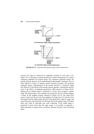
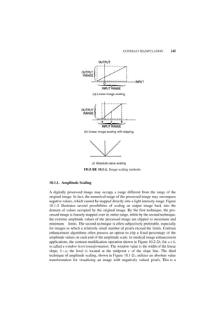
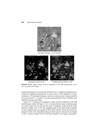
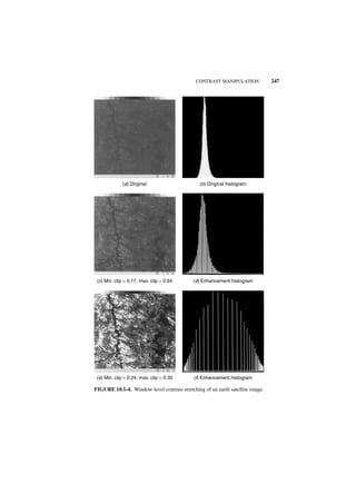
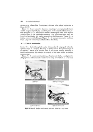
![CONTRAST MANIPULATION 249
(a ) Square function (b ) Square output
(c ) Cube function (d ) Cube output
FIGURE 10.1-6. Square and cube contrast modification of the jet_mon image.
The histogram of the image is shown in Figure 10.1-5b. Examination of the
histogram of the image reveals that the image contains relatively few low- or high-
amplitude pixels. Consequently, applying the window-level contrast stretching
function of Figure 10.1-5c results in the image of Figure 10.1-5d, which possesses
better visual contrast but does not exhibit noticeable visual clipping.
Consideration will now be given to several nonlinear point transformations, some
of which will be seen to improve visual contrast, while others clearly impair visual
contrast.
Figures 10.1-6 and 10.1-7 provide examples of power law point transformations
in which the processed image is defined by
p
G ( j, k ) = [ F ( j, k ) ] (10.1-1)](https://image.slidesharecdn.com/digitalimageprocessing-120319064358-phpapp01/85/Digital-image-processing-257-320.jpg)
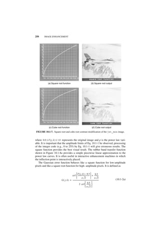
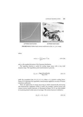

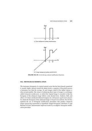
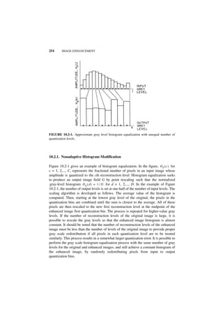
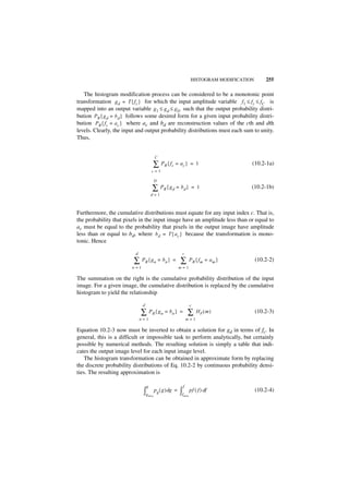
![256
TABLE 10.2-1. Histogram Modification Transfer Functions
Output Probability Density Model Transfer Functiona
Uniform 1 -
p g ( g ) = ---------------------------- g min ≤ g ≤ g max g = ( g max – g min )Pf ( f ) + g min
g max – g min
Exponential p g ( g ) = α exp { – α ( g – g min ) } g ≤ g min 1
g = g min – --- ln { 1 – Pf ( f ) }
α
2 1⁄2
g – g min ( g – g min ) 2
Rayleigh - -
p g ( g ) = ------------------- exp – -------------------------- g ≥ g min 1 -
g = g min + 2α ln --------------------
2 2
α 2α 1 – Pf( f )
–2 ⁄ 3 3
g
1 ---------------------------- 1⁄3 1⁄3 1⁄3
Hyperbolic -
p g ( g ) = -- - g = g max – g min [ P f ( f ) ] + g max
(Cube root) 3 g 1 ⁄ 3 – g1 ⁄ 3
max min
1 g max P f ( f )
Hyperbolic p g ( g ) = ------------------------------------------------------------- g = g min -----------
g [ ln { g max } – ln { g min } ] g
(Logarithmic) min
aThe cumulative probability distribution P (f), of the input image is approximated by its cumulative histogram:
f
j
pf ( f ) ≈ ∑ HF ( m )
m=0](https://image.slidesharecdn.com/digitalimageprocessing-120319064358-phpapp01/85/Digital-image-processing-264-320.jpg)
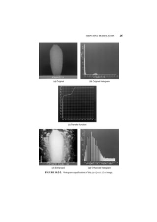

![HISTOGRAM MODIFICATION 259
(a ) Original
(b) Transfer function (c ) Histogram equalized
FIGURE 10.2-3. Histogram equalization of the jet_mon image.
made spatially adaptive by applying histogram modification to each pixel based on
the histogram of pixels within a moving window neighborhood. This technique is
obviously computationally intensive, as it requires histogram generation, mapping
function computation, and mapping function application at each pixel.
Pizer et al. (9) have proposed an adaptive histogram equalization technique in
which histograms are generated only at a rectangular grid of points and the mappings
at each pixel are generated by interpolating mappings of the four nearest grid points.
Figure 10.2-5 illustrates the geometry. A histogram is computed at each grid point in
a window about the grid point. The window dimension can be smaller or larger than
the grid spacing. Let M00, M01, M10, M11 denote the histogram modification map-
pings generated at four neighboring grid points. The mapping to be applied at pixel
F(j, k) is determined by a bilinear interpolation of the mappings of the four nearest
grid points as given by
M = a [ bM00 + ( 1 – b )M 10 ] + ( 1 – a ) [ bM 01 + ( 1 – b )M 11 ] (10.2-8a)](https://image.slidesharecdn.com/digitalimageprocessing-120319064358-phpapp01/85/Digital-image-processing-267-320.jpg)
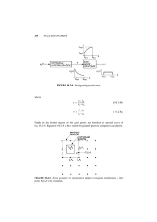
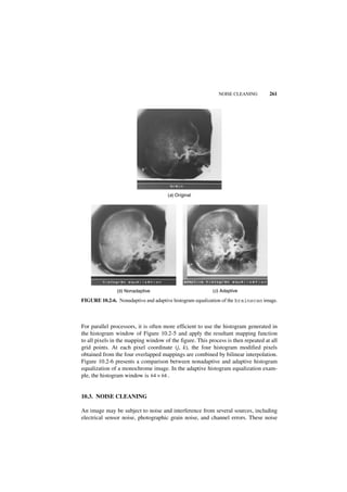
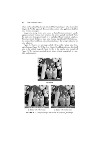
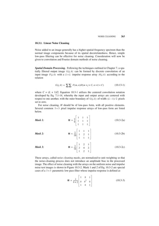
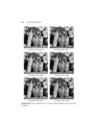
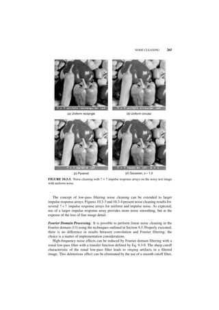
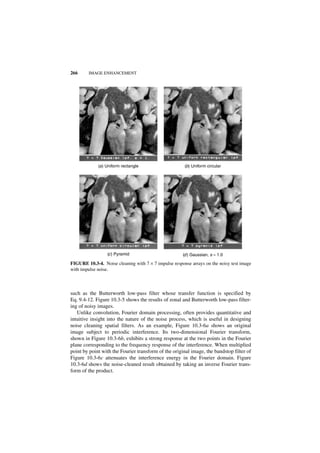
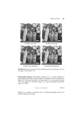
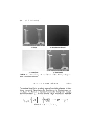
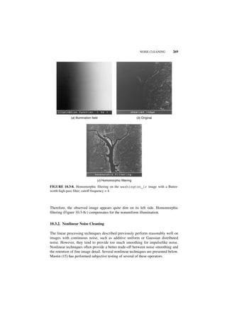
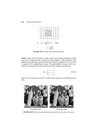
![NOISE CLEANING 271
The outlier operator can be extended straightforwardly to larger windows. Davis
and Rosenfeld (16) have suggested a variant of the outlier technique in which the
center pixel in a window is replaced by the average of its k neighbors whose ampli-
tudes are closest to the center pixel.
Median Filter. Median filtering is a nonlinear signal processing technique devel-
oped by Tukey (17) that is useful for noise suppression in images. In one-dimen-
sional form, the median filter consists of a sliding window encompassing an odd
number of pixels. The center pixel in the window is replaced by the median of the
pixels in the window. The median of a discrete sequence a1, a2,..., aN for N odd is
that member of the sequence for which (N – 1)/2 elements are smaller or equal in
value and (N – 1)/2 elements are larger or equal in value. For example, if the values
of the pixels within a window are 0.1, 0.2, 0.9, 0.4, 0.5, the center pixel would be
replaced by the value 0.4, which is the median value of the sorted sequence 0.1, 0.2,
0.4, 0.5, 0.9. In this example, if the value 0.9 were a noise spike in a monotonically
increasing sequence, the median filter would result in a considerable improvement.
On the other hand, the value 0.9 might represent a valid signal pulse for a wide-
bandwidth sensor, and the resultant image would suffer some loss of resolution.
Thus, in some cases the median filter will provide noise suppression, while in other
cases it will cause signal suppression.
Figure 10.3-11 illustrates some examples of the operation of a median filter and a
mean (smoothing) filter for a discrete step function, ramp function, pulse function,
and a triangle function with a window of five pixels. It is seen from these examples
that the median filter has the usually desirable property of not affecting step func-
tions or ramp functions. Pulse functions, whose periods are less than one-half the
window width, are suppressed. But the peak of the triangle is flattened.
Operation of the median filter can be analyzed to a limited extent. It can be
shown that the median of the product of a constant K and a sequence f ( j ) is
MED { K [ f ( j ) ] } = K [ MED { f ( j ) } ] (10.3-7)
However, for two arbitrary sequences f ( j ) and g ( j ), it does not follow that the
median of the sum of the sequences is equal to the sum of their medians. That is, in
general,
MED { f ( j ) + g ( j ) } ≠ MED { f ( j ) } + MED { g ( j ) } (10.3-8)
The sequences 0.1, 0.2, 0.3, 0.4, 0.5 and 0.1, 0.2, 0.3, 0.2, 0.1 are examples for
which the additive linearity property does not hold.
There are various strategies for application of the median filter for noise suppres-
sion. One method would be to try a median filter with a window of length 3. If there
is no significant signal loss, the window length could be increased to 5 for median](https://image.slidesharecdn.com/digitalimageprocessing-120319064358-phpapp01/85/Digital-image-processing-279-320.jpg)
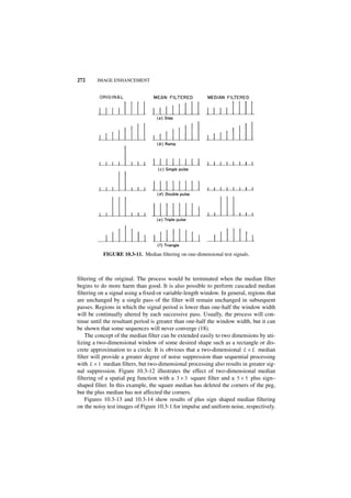
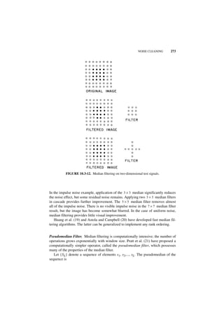
![274 IMAGE ENHANCEMENT
(a) 3 × 3 median filter (b) 3 × 3 cascaded median filter
(c) 5 × 5 median filter (d) 7 × 7 median filter
FIGURE 10.3-13. Median filtering on the noisy test image with uniform noise.
PMED { S L } = ( 1 ⁄ 2 )MAXIMIN { S L } + ( 1 ⁄ 2 )MINIMAX { S L } (10.3-9)
where for M = (L + 1)/2
MAXIMIN { S L } = MAX { [ MIN ( s 1, …, s M ) ], [ MIN ( s 2, …, s M + 1 ) ]
…, [ MIN ( sL – M + 1, …, sL ) ] } (10.3-10a)
MINIMAX { S L } = MIN { [ MAX ( s 1, …, s M ) ], [ MAX ( s 2, …, s M + 1 ) ]
…, [ MAX ( s L – M + 1, …, s L ) ] } (10.3-10b)](https://image.slidesharecdn.com/digitalimageprocessing-120319064358-phpapp01/85/Digital-image-processing-282-320.jpg)
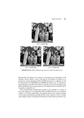
![276 IMAGE ENHANCEMENT
y1
·
·
·
x 1 … xM … xC
·
·
·
yR
Let the sequences {XC} and {YR} denote the elements along the horizontal and ver-
tical axes of the window, respectively. Note that the element xM is common to both
sequences. Then the plus-shaped pseudomedian can be defined as
PMED { S E } = ( 1 ⁄ 2 )MAX [ MAXIMIN { X C }, MAXIMIN { Y R } ]
+ ( 1 ⁄ 2 ) MIN [ MINIMAX { XC }, MINIMAX { Y R } ]
(10.3-11)
The MAXIMIN operator in one- or two-dimensional form is useful for removing
bright impulse noise but has little or no effect on dark impulse noise. Conversely,
the MINIMAX operator does a good job in removing dark, but not bright, impulse
noise. A logical conclusion is to cascade the operators.
Figure 10.3-16 shows the results of MAXIMIN, MINIMAX, and pseudomedian
filtering on an image subjected to salt and pepper noise. As observed, the
MAXIMIN operator reduces the salt noise, while the MINIMAX operator reduces
the pepper noise. The pseudomedian provides attenuation for both types of noise.
The cascade MINIMAX and MAXIMIN operators, in either order, show excellent
results.
Wavelet De-noising. Section 8.4-3 introduced wavelet transforms. The usefulness
of wavelet transforms for image coding derives from the property that most of the
energy of a transformed image is concentrated in the trend transform components
rather than the fluctuation components (22). The fluctuation components may be
grossly quantized without serious image degradation. This energy compaction prop-
erty can also be exploited for noise removal. The concept, called wavelet de-noising
(22,23), is quite simple. The wavelet transform coefficients are thresholded such
that the presumably noisy, low-amplitude coefficients are set to zero.](https://image.slidesharecdn.com/digitalimageprocessing-120319064358-phpapp01/85/Digital-image-processing-284-320.jpg)
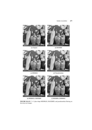
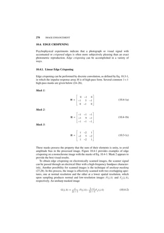
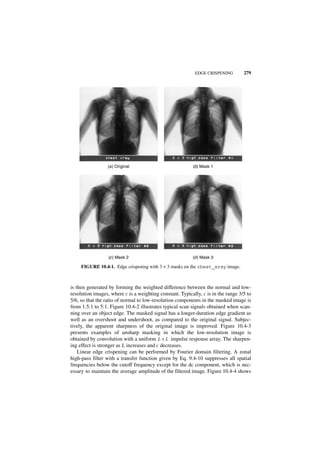
![280 IMAGE ENHANCEMENT
FIGURE 10.4-2. Waveforms in an unsharp masking image enhancement system.
the result of zonal high-pass filtering of an image. Zonal high-pass filtering often
causes ringing in a filtered image. Such ringing can be reduced significantly by utili-
zation of a high-pass filter with a smooth cutoff response. One such filter is the
Butterworth high-pass filter, whose transfer function is defined by Eq. 9.4-13.
Figure 10.4-4 shows the results of zonal and Butterworth high-pass filtering. In
both examples, the filtered images are biased to a midgray level for display.
10.4.2. Statistical Differencing
Another form of edge crispening, called statistical differencing (29, p. 100),
involves the generation of an image by dividing each pixel value by its estimated
standard deviation D ( j, k ) according to the basic relation
F ( j, k )
G ( j, k ) = ----------------- (10.4-3)
D ( j, k )
where the estimated standard deviation
j+w k+w 1⁄2
1 2
D ( j, k ) = ----
W
- ∑ ∑ [ F ( m, n ) – M ( m, n ) ] (10.4-4)
m = j–w n = k–w](https://image.slidesharecdn.com/digitalimageprocessing-120319064358-phpapp01/85/Digital-image-processing-288-320.jpg)
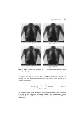
![282 IMAGE ENHANCEMENT
(a) Zonal filtering (b) Butterworth filtering
FIGURE 10.4-4. Zonal and Butterworth high-pass filtering on the chest_xray image;
cutoff frequency = 32.
Wallis (30) has suggested a generalization of the statistical differencing operator
in which the enhanced image is forced to a form with desired first- and second-order
moments. The Wallis operator is defined by
A max D d
G ( j, k ) = [ F ( j, k ) – M ( j, k ) ] ------------------------------------------ + [ pM d + ( 1 – p )M ( j, k ) ]
- (10.4-6)
A max D ( j, k ) + D d
where Md and Dd represent desired average mean and standard deviation factors,
Amax is a maximum gain factor that prevents overly large output values when
D ( j, k ) is small and 0.0 ≤ p ≤ 1.0 is a mean proportionality factor controlling the
background flatness of the enhanced image.
The Wallis operator can be expressed in a more general form as
G ( j, k ) = [ F ( j, k ) – M ( j, k ) ]A ( j, k ) + B ( j, k ) (10.4-7)
where A ( j, k ) is a spatially dependent gain factor and B ( j, k ) is a spatially depen-
dent background factor. These gain and background factors can be derived directly
from Eq. 10.4-4, or they can be specified in some other manner. For the Wallis oper-
ator, it is convenient to specify the desired average standard deviation Dd such that
the spatial gain ranges between maximum Amax and minimum Amin limits. This can
be accomplished by setting Dd to the value](https://image.slidesharecdn.com/digitalimageprocessing-120319064358-phpapp01/85/Digital-image-processing-290-320.jpg)
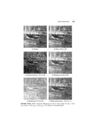
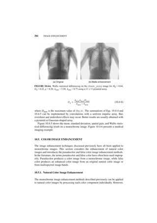

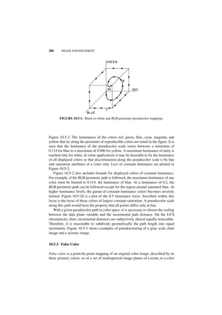
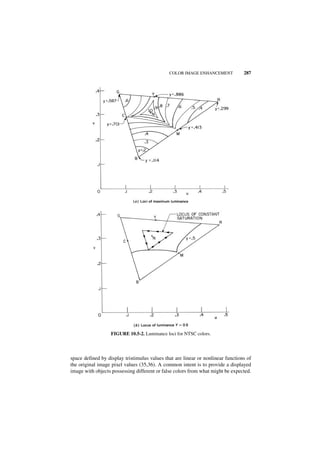
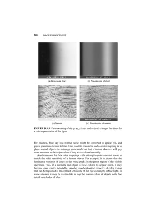
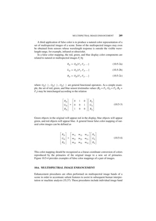
![290 IMAGE ENHANCEMENT
(a) Infrared band (b) Blue band
(c) R = infrared, G = 0, B = blue (d ) R = infrared, G = 1/2 [infrared + blue], B = blue
FIGURE 10.5-4. False coloring of multispectral images. See insert for a color representation
of this figure.
enhancement techniques, such as contrast stretching, noise cleaning, and edge crisp-
ening, as described earlier. Other methods, considered in this section, involve the
joint processing of multispectral image bands.
Multispectral image bands can be subtracted in pairs according to the relation
D m, n ( j, k ) = Fm ( j, k ) – Fn ( j, k ) (10.6-1)
in order to accentuate reflectivity variations between the multispectral bands. An
associated advantage is the removal of any unknown but common bias components
that may exist. Another simple but highly effective means of multispectral image
enhancement is the formation of ratios of the image bands. The ratio image between
the mth and nth multispectral bands is defined as](https://image.slidesharecdn.com/digitalimageprocessing-120319064358-phpapp01/85/Digital-image-processing-298-320.jpg)
![MULTISPECTRAL IMAGE ENHANCEMENT 291
F m ( j, k )
Rm, n ( j, k ) = -------------------
- (10.6-2)
F n ( j, k )
It is assumed that the image bands are adjusted to have nonzero pixel values. In
many multispectral imaging systems, the image band Fn ( j, k ) can be modeled by
the product of an object reflectivity function R n ( j, k ) and an illumination function
I ( j, k ) that is identical for all multispectral bands. Ratioing of such imagery provides
an automatic compensation of the illumination factor. The ratio
F m ( j, k ) ⁄ [ F n ( j, k ) ± ∆ ( j, k ) ], for which ∆ ( j, k ) represents a quantization level uncer-
tainty, can vary considerably if F n ( j, k ) is small. This variation can be reduced
significantly by forming the logarithm of the ratios defined by (24)
L m, n ( j, k ) = log { R m, n ( j, k ) } = log { F m ( j, k ) } – log { F n ( j, k ) } (10.6-3)
There are a total of N(N – 1) different difference or ratio pairs that may be formed
from N multispectral bands. To reduce the number of combinations to be consid-
ered, the differences or ratios are often formed with respect to an average image
field:
N
1
A ( j, k ) = ---
N
- ∑ F n ( j, k ) (10.6-4)
n=1
Unitary transforms between multispectral planes have also been employed as a
means of enhancement. For N image bands, a N × 1 vector
F 1 ( j, k )
F 2 ( j, k )
·
x = (10.6-5)
·
·
F N ( j, k )
is formed at each coordinate (j, k). Then, a transformation
y = Ax (10.6-6)](https://image.slidesharecdn.com/digitalimageprocessing-120319064358-phpapp01/85/Digital-image-processing-299-320.jpg)
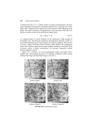
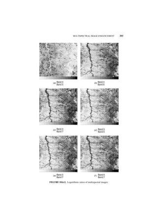
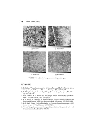


![GENERAL IMAGE RESTORATION MODELS 299
where O G { · } is an operator modeling the image digitization process.
A digital image restoration system that follows produces an output array
(i)
FK ( k 1, k 2, tj ) by the transformation
(i ) ( i)
F K ( k 1, k 2, t j ) = O R { FS ( m 1, m2, t j ) } (11.1-3)
where O R { · } represents the designed restoration operator. Next, the output samples
of the digital restoration system are interpolated by the image display system to pro-
duce a continuous image estimate F ( i ) ( x, y, t j ). This operation is governed by the
ˆ
I
relation
ˆ (i) (i)
FI ( x, y, t j ) = O D { FK ( k 1, k 2, tj ) } (11.1-4)
where O D { · } models the display transformation.
The function of the digital image restoration system is to compensate for degra-
dations of the physical imaging system, the digitizer, and the image display system
(i)
to produce an estimate of a hypothetical ideal image field FI ( x, y, t j ) that would be
displayed if all physical elements were perfect. The perfect imaging system would
produce an ideal image field modeled by
(i) ∞ t
FI ( x, y, t j ) = O I ∫ ∫ j C ( x, y, t, λ )U i ( t, λ ) dt dλ (11.1-5)
0 tj – T
where U i ( t, λ ) is a desired temporal and spectral response function, T is the observa-
tion period, and O I { · } is a desired point and spatial response function.
Usually, it will not be possible to restore perfectly the observed image such that
the output image field is identical to the ideal image field. The design objective of
the image restoration processor is to minimize some error measure between
(i)
FI ( x, y, t j ) and F ( i ) ( x, y, t j ). The discussion here is limited, for the most part, to a
ˆ
I
consideration of techniques that minimize the mean-square error between the ideal
and estimated image fields as defined by
(i ) ˆ (i ) 2
E i = E [ F I ( x, y, t j ) – F I ( x, y, t j ) ] (11.1-6)
where E { · } denotes the expectation operator. Often, it will be desirable to place
side constraints on the error minimization, for example, to require that the image
estimate be strictly positive if it is to represent light intensities that are positive.
Because the restoration process is to be performed digitally, it is often more con-
venient to restrict the error measure to discrete points on the ideal and estimated
image fields. These discrete arrays are obtained by mathematical models of perfect
image digitizers that produce the arrays](https://image.slidesharecdn.com/digitalimageprocessing-120319064358-phpapp01/85/Digital-image-processing-307-320.jpg)
![300 IMAGE RESTORATION MODELS
(i) (i)
FI ( n 1, n 2, t j ) = F I ( x, y, tj )δ ( x – n 1 ∆, y – n 2 ∆ ) (11.1-7a)
ˆ (i) ˆ (i)
FI ( n 1, n 2, t j ) = F I ( x, y, tj )δ ( x – n 1 ∆, y – n 2 ∆ ) (11.1-7b)
It is assumed that continuous image fields are sampled at a spatial period ∆ satisfy-
ing the Nyquist criterion. Also, quantization error is assumed negligible. It should be
noted that the processes indicated by the blocks of Figure 11.1-1 above the dashed
division line represent mathematical modeling and are not physical operations per-
formed on physical image fields and arrays. With this discretization of the continu-
ous ideal and estimated image fields, the corresponding mean-square restoration
error becomes
(i ) ˆ (i) 2
E i = E [ F I ( n 1, n 2, t j ) – F I ( n 1, n 2, tj ) ] (11.1-8)
With the relationships of Figure 11.1-1 quantitatively established, the restoration
problem may be formulated as follows:
(i)
Given the sampled observation F S ( m 1, m 2, t j ) expressed in terms of the
image light distribution C ( x, y, t, λ ), determine the transfer function O K { · }
(i ) ˆ (i)
that minimizes the error measure between F I ( x, y, t j ) and FI ( x, y, t j ) subject
to desired constraints.
There are no general solutions for the restoration problem as formulated above
because of the complexity of the physical imaging system. To proceed further, it is
necessary to be more specific about the type of degradation and the method of resto-
ration. The following sections describe models for the elements of the generalized
imaging system of Figure 11.1-1.
11.2. OPTICAL SYSTEMS MODELS
One of the major advances in the field of optics during the past 40 years has been the
application of system concepts to optical imaging. Imaging devices consisting of
lenses, mirrors, prisms, and so on, can be considered to provide a deterministic
transformation of an input spatial light distribution to some output spatial light dis-
tribution. Also, the system concept can be extended to encompass the spatial propa-
gation of light through free space or some dielectric medium.
In the study of geometric optics, it is assumed that light rays always travel in a
straight-line path in a homogeneous medium. By this assumption, a bundle of rays
passing through a clear aperture onto a screen produces a geometric light projection
of the aperture. However, if the light distribution at the region between the light and](https://image.slidesharecdn.com/digitalimageprocessing-120319064358-phpapp01/85/Digital-image-processing-308-320.jpg)
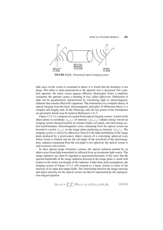

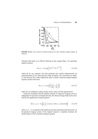

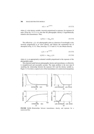
![PHOTOGRAPHIC PROCESS MODELS 307
FIGURE 11.3-3. H & D curves for a reversal film as a function of development time.
as a function of exposure. It is to be noted that the curve is highly nonlinear except
for a relatively narrow region in the lower exposure range. In Figure 11.3-2b, the
curve of Figure 11.3-2a has been replotted as transmittance versus the logarithm of
exposure. An approximate linear relationship is found to exist between transmit-
tance and the logarithm of exposure, but operation in this exposure region is usually
of little use in imaging systems. The parameter of interest in photography is the pho-
tographic density variable dx, which is plotted as a function of exposure and loga-
rithm of exposure in Figure 11.3-2c and 11.3-2d. The plot of density versus
logarithm of exposure is known as the H & D curve after Hurter and Driffield, who
performed fundamental investigations of the relationships between density and
exposure. Figure 11.3-3 is a plot of the H & D curve for a reversal type of film. In
Figure 11.3-2d, the central portion of the curve, which is approximately linear, has
been approximated by the line defined by
d x = γ [ log 10 X ( C ) – KF ] (11.3-7)
where γ represents the slope of the line and KF denotes the intercept of the line with
the log exposure axis. The slope of the curve γ (gamma,) is a measure of the contrast
of the film, while the factor KF is a measure of the film speed; that is, a measure of
the base exposure required to produce a negative in the linear region of the H & D
curve. If the exposure is restricted to the linear portion of the H & D curve, substitu-
tion of Eq. 11.3-7 into Eq. 11.3-3 yields a transmittance function
– γD ( λ )
τ ( λ ) = Kτ ( λ ) [ X ( C ) ] (11.3-8a)
where
γK F D ( λ )
K τ ( λ ) ≡ 10 (11.3-8b)](https://image.slidesharecdn.com/digitalimageprocessing-120319064358-phpapp01/85/Digital-image-processing-315-320.jpg)
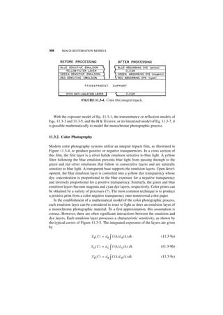
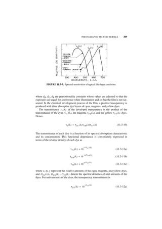
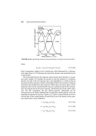
![PHOTOGRAPHIC PROCESS MODELS 311
FIGURE 11.3-7. H & D curves for a typical reversal color film.
where γC , γM , γ Y , representing the slopes of the curves in the linear region, are
called dye layer gammas.
The spectral energy distribution of light passing through a developed transpar-
ency is the product of the transparency transmittance and the incident illumination
spectral energy distribution E ( λ ) as given by
– [ cD NC ( λ ) + mD NM ( λ ) + yD NY ( λ ) ]
CT ( λ ) = E ( λ )10 (11.3-14)
Figure 11.3-8 is a block diagram of the complete color film recording and reproduc-
tion process. The original light with distribution C ( λ ) and the light passing through
the transparency C T ( λ ) at a given resolution element are rarely identical. That is, a
spectral match is usually not achieved in the photographic process. Furthermore, the
lights C and CT usually do not even provide a colorimetric match.](https://image.slidesharecdn.com/digitalimageprocessing-120319064358-phpapp01/85/Digital-image-processing-319-320.jpg)
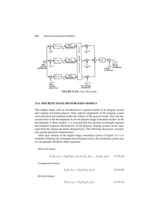
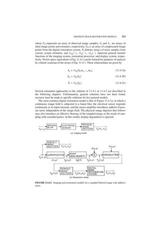
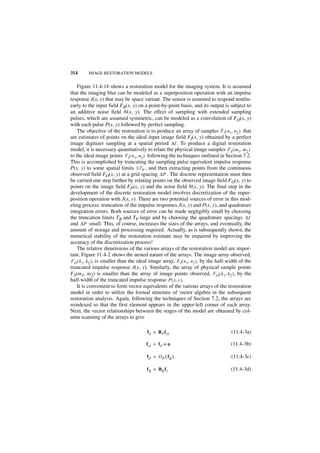
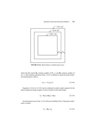
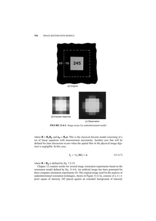

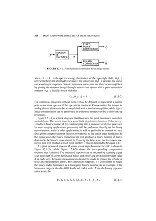
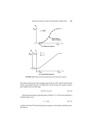
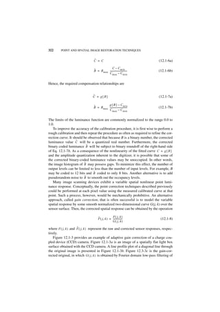
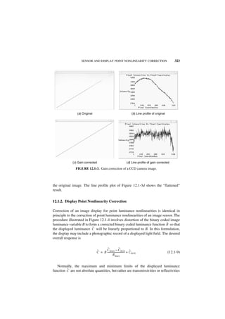
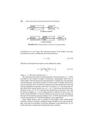
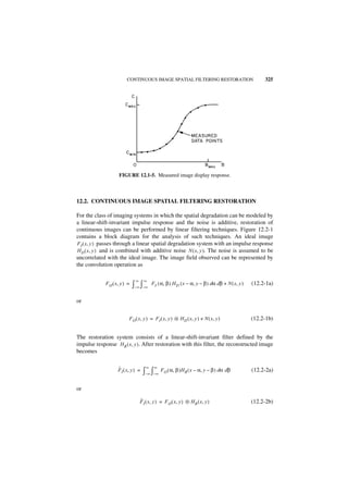
![326 POINT AND SPATIAL IMAGE RESTORATION TECHNIQUES
FIGURE 12.2-1. Continuous image restoration model.
Substitution of Eq. 12.2-lb into Eq. 12.2-2b yields
ˆ
F I ( x, y ) = [ F I ( x, y ) ᭺ H D ( x, y ) + N ( x, y ) ] ᭺ H R ( x, y )
ء ء (12.2-3)
It is analytically convenient to consider the reconstructed image in the Fourier trans-
form domain. By the Fourier transform convolution theorem,
ˆ
F I ( ω x, ω y ) = [ F I ( ω x, ω y )H D ( ω x, ω y ) + N ( ω x, ω y ) ]H R ( ω x, ω y ) (12.2-4)
ˆ
where F I ( ω x, ω y ), F I ( ω x, ω y ), N ( ω x, ω y ), HD ( ω x, ω y ), H R ( ω x, ω y ) are the two-dimen-
ˆ
sional Fourier transforms of FI ( x, y ), F I ( x, y ) N ( x, y ), H D ( x, y ), H R ( x, y ), respec-
,
tively.
The following sections describe various types of continuous image restoration
filters.
12.2.1. Inverse Filter
The earliest attempts at image restoration were based on the concept of inverse fil-
tering, in which the transfer function of the degrading system is inverted to yield a
restored image (8–12). If the restoration inverse filter transfer function is chosen so
that
1
H R ( ω x, ω y ) = ---------------------------
- (12.2-5)
H D ( ω x, ω y )
then the spectrum of the reconstructed image becomes
N ( ω x, ω y )
ˆ
F I ( ω x, ω y ) = F I ( ω x, ω y ) + ---------------------------
- (12.2-6)
H D ( ω x, ω y )](https://image.slidesharecdn.com/digitalimageprocessing-120319064358-phpapp01/85/Digital-image-processing-333-320.jpg)
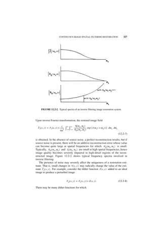
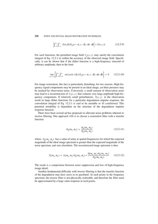
![CONTINUOUS IMAGE SPATIAL FILTERING RESTORATION 329
12.2.2. Wiener Filter
It should not be surprising that inverse filtering performs poorly in the presence of
noise because the filter design ignores the noise process. Improved restoration qual-
ity is possible with Wiener filtering techniques, which incorporate a priori statistical
knowledge of the noise field (13–17).
In the general derivation of the Wiener filter, it is assumed that the ideal image
FI ( x, y ) and the observed image F O ( x, y ) of Figure 12.2-1 are samples of two-
dimensional, continuous stochastic fields with zero-value spatial means. The
impulse response of the restoration filter is chosen to minimize the mean-square res-
toration error
ˆ 2
E = E { [ F I ( x, y ) – FI ( x, y ) ] } (12.2-13)
The mean-square error is minimized when the following orthogonality condition is
met (13):
ˆ
E { [ FI ( x, y ) – FI ( x, y ) ]F O ( x′, y′ ) } = 0 (12.2-14)
for all image coordinate pairs ( x, y ) and ( x′, y′ ). Upon substitution of Eq. 12.2-2a
for the restored image and some linear algebraic manipulation, one obtains
∞ ∞
E { FI ( x, y )FO ( x, y ) } = ∫–∞ ∫–∞ E { FO ( α, β )FO ( x′, y′ ) }HR ( x – α, y – β ) dα dβ (12.2-15)
Under the assumption that the ideal image and observed image are jointly stationary,
the expectation terms can be expressed as covariance functions, as in Eq. 1.4-8. This
yields
∞ ∞
K F F ( x – x′, y – y′ ) =
I O ∫– ∞ ∫– ∞ K F O FO
( α – x′, β – y′ )H R ( x – α, y – β ) dα dβ (12.2-16)
Then, taking the two-dimensional Fourier transform of both sides of Eq. 12.2-16 and
solving for H R ( ω x, ω y ) , the following general expression for the Wiener filter trans-
fer function is obtained:
W F F ( ω x, ω y )
HR ( ω x, ω y ) = -------------------------------------
I O
(12.2-17)
W F F ( ω x, ω y )
O O
In the special case of the additive noise model of Figure 12.2-1:](https://image.slidesharecdn.com/digitalimageprocessing-120319064358-phpapp01/85/Digital-image-processing-336-320.jpg)
![330 POINT AND SPATIAL IMAGE RESTORATION TECHNIQUES
*
WF F ( ω x, ω y ) = HD ( ω x, ω y )W F ( ω x, ω y ) (12.2-18a)
I O I
2
WF ( ω x, ω y ) = H D ( ω x, ω y ) W F ( ω x, ω y ) + WN ( ω x, ω y ) (12.2-18b)
O FO I
This leads to the additive noise Wiener filter
*
H D ( ω x, ω y )W F ( ω x, ω y )
H R ( ω x, ω y ) = ----------------------------------------------------------------------------------------------------
I
- (12.2-19a)
2
H D ( ω x, ω y ) W F ( ω x, ω y ) + W N ( ω x, ω y )
I
or
*
HD ( ω x, ω y )
H R ( ω x, ω y ) = --------------------------------------------------------------------------------------------------------
- (12.2-19b)
2
H D ( ω x, ω y ) + W N ( ω x, ω y ) ⁄ W F ( ω x, ω y )
I
In the latter formulation, the transfer function of the restoration filter can be
expressed in terms of the signal-to-noise power ratio
W F ( ω x, ω y )
SNR ( ω x, ω y ) ≡ -----------------------------
I
- (12.2-20)
W N ( ω x, ω y )
at each spatial frequency. Figure 12.2-3 shows cross-sectional sketches of a typical
ideal image spectrum, noise spectrum, blur transfer function, and the resulting
Wiener filter transfer function. As noted from the figure, this version of the Wiener
filter acts as a bandpass filter. It performs as an inverse filter at low spatial frequen-
cies, and as a smooth rolloff low-pass filter at high spatial frequencies.
Equation 12.2-19 is valid when the ideal image and observed image stochastic
processes are zero mean. In this case, the reconstructed image Fourier transform is
ˆ
F I ( ω x, ω y ) = H R ( ω x, ω y )F O ( ω x, ω y ) (12.2-21)
If the ideal image and observed image means are nonzero, the proper form of the
reconstructed image Fourier transform is
ˆ
F I ( ω x, ω y ) = H R ( ω x, ω y ) [ F O ( ω x, ω y ) – M O ( ω x, ω y ) ] + MI ( ω x, ω y ) (12.2-22a)
where
M O ( ω x, ω y ) = H D ( ω x, ω y )M I ( ω x, ω y ) + MN ( ω x, ω y ) (12.2-22b)](https://image.slidesharecdn.com/digitalimageprocessing-120319064358-phpapp01/85/Digital-image-processing-337-320.jpg)
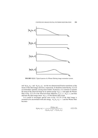
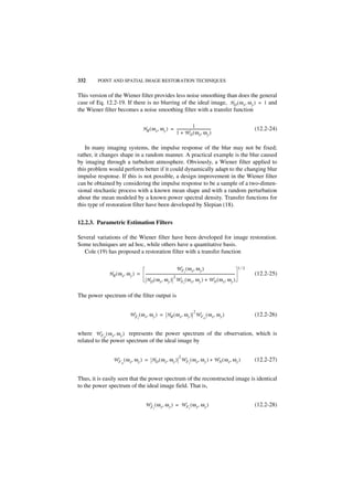
![CONTINUOUS IMAGE SPATIAL FILTERING RESTORATION 333
For this reason, the restoration filter defined by Eq. 12.2-25 is called the image
power-spectrum filter. In contrast, the power spectrum for the reconstructed image
as obtained by the Wiener filter of Eq. 12.2-19 is
2 2
H D ( ω x, ω y ) [ W F ( ω x, ω y ) ]
WF ( ω x, ω y ) = ----------------------------------------------------------------------------------------------------
ˆI
I
- (12.2-29)
2
H D ( ω x, ω y ) W F ( ω x, ω y ) + W N ( ω x, ω y )
I
In this case, the power spectra of the reconstructed and ideal images become identi-
cal only for a noise-free observation. Although equivalence of the power spectra of
the ideal and reconstructed images appears to be an attractive feature of the image
power-spectrum filter, it should be realized that it is more important that the Fourier
spectra (Fourier transforms) of the ideal and reconstructed images be identical
because their Fourier transform pairs are unique, but power-spectra transform pairs
are not necessarily unique. Furthermore, the Wiener filter provides a minimum
mean-square error estimate, while the image power-spectrum filter may result in a
large residual mean-square error.
Cole (19) has also introduced a geometrical mean filter, defined by the transfer
function
–S H ∗ ( ω x, ω y )W F ( ω x, ω y )
D
1–S
H R ( ω x, ω y ) = [ H D ( ω x, ω y ) ] ----------------------------------------------------------------------------------------------------
I
- (12.2-30)
2
H D ( ω x, ω y ) W F ( ω x, ω y ) + W N ( ω x, ω y )
I
where 0 ≤ S ≤ 1 is a design parameter. If S = 1 ⁄ 2 and H D = H ∗ , the geometrical
D
mean filter reduces to the image power-spectrum filter as given in Eq. 12.2-25.
Hunt (20) has developed another parametric restoration filter, called the con-
strained least-squares filter, whose transfer function is of the form
H ∗ ( ω x, ω y )
D
H R ( ω x, ω y ) = ------------------------------------------------------------------------
- (12.2-31)
2 2
H D ( ω x, ω y ) + γ C ( ω x, ω y )
where γ is a design constant and C ( ω x, ω y ) is a design spectral variable. If γ = 1
2
and C ( ω x, ω y ) is set equal to the reciprocal of the spectral signal-to-noise power
ratio of Eq. 12.2-20, the constrained least-squares filter becomes equivalent to the
Wiener filter of Eq. 12.2-19b. The spectral variable can also be used to minimize
higher-order derivatives of the estimate.
12.2.4. Application to Discrete Images
The inverse filtering, Wiener filtering, and parametric estimation filtering tech-
niques developed for continuous image fields are often applied to the restoration of](https://image.slidesharecdn.com/digitalimageprocessing-120319064358-phpapp01/85/Digital-image-processing-340-320.jpg)
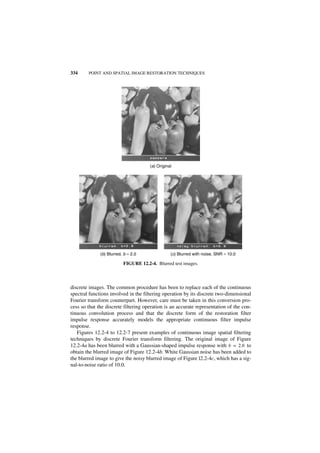
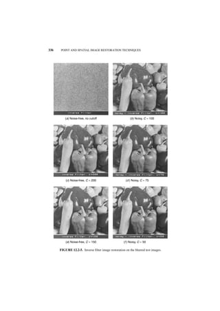
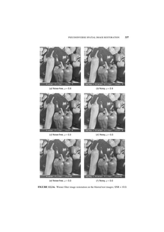
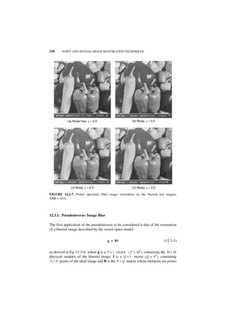
![PSEUDOINVERSE SPATIAL IMAGE RESTORATION 339
on the impulse function. If the physical sample period and the quadrature represen-
tation period are identical, P will be smaller than Q, and the system of equations will
be underdetermined. By oversampling the blurred image, it is possible to force
P > Q or even P = Q . In either case, the system of equations is called overdeter-
mined. An overdetermined set of equations can also be obtained if some of the
elements of the ideal image vector can be specified through a priori knowledge. For
example, if the ideal image is known to contain a limited size object against a black
background (zero luminance), the elements of f beyond the limits may be set to zero.
ˆ
In discrete form, the restoration problem reduces to finding a solution f to Eq.
12.3-1 in the sense that
ˆ
Bf = g (12.3-2)
Because the vector g is determined by physical sampling and the elements of B are
specified independently by system modeling, there is no guarantee that a f even ˆ
exists to satisfy Eq. 12.3-2. If there is a solution, the system of equations is said to be
consistent; otherwise, the system of equations is inconsistent.
In Appendix 1 it is shown that inconsistency in the set of equations of Eq. 12.3-1
can be characterized as
g = Bf + e { f } (12.3-3)
where e { f } is a vector of remainder elements whose value depends on f. If the set
of equations is inconsistent, a solution of the form
ˆ = Wg
f (12.3-4)
is sought for which the linear operator W minimizes the least-squares modeling
error
E M = [ e { ˆ } ] [ e { ˆ } ] = [ g – Bf ] [ g – Bf ]
ˆ ˆ
T T
f f (12.3-5)
This error is shown, in Appendix 1, to be minimized when the operator W = B$ is
set equal to the least-squares inverse of B. The least-squares inverse is not necessar-
ily unique. It is also proved in Appendix 1 that the generalized inverse operator
W = B–, which is a special case of the least-squares inverse, is unique, minimizes
the least-squares modeling error, and simultaneously provides a minimum norm
estimate. That is, the sum of the squares of ˆ is a minimum for all possible mini-
f
mum least-square error estimates. For the restoration of image blur, the generalized
inverse provides a lowest-intensity restored image.](https://image.slidesharecdn.com/digitalimageprocessing-120319064358-phpapp01/85/Digital-image-processing-346-320.jpg)
![340 POINT AND SPATIAL IMAGE RESTORATION TECHNIQUES
If Eq. 12.3-1 represents a consistent set of equations, one or more solutions may
exist for Eq. 12.3-2. The solution commonly chosen is the estimate that minimizes
the least-squares estimation error defined in the equivalent forms
EE = ( f – ˆ) ( f – ˆ)
T
f f (12.3-6a)
E E = tr { ( f – f ) ( f – ˆ ) }
ˆ T
f (12.3-6b)
In Appendix 1 it is proved that the estimation error is minimum for a generalized
inverse (W = B–) estimate. The resultant residual estimation error then becomes
T –
E E = f [ I – [ B B ] ]f (12.3-7a)
or
T –
E E = tr { ff [ I – [ B B ] ] } (12.3-7b)
The estimate is perfect, of course, if B–B = I.
Thus, it is seen that the generalized inverse is an optimal solution, in the sense
defined previously, for both consistent and inconsistent sets of equations modeling
image blur. From Eq. 5.5-5, the generalized inverse has been found to be algebra-
ically equivalent to
– T –1 T
B = [B B] B (12.3-8a)
if the P × Q matrix B is of rank Q. If B is of rank P, then
– T T –1
B = B [B B] (12.3-8b)
For a consistent set of equations and a rank Q generalized inverse, the estimate
–1
ˆ = B – g = B – Bf = [ [ B T B ] B T ]Bf = f
f (12.3-9)
is obviously perfect. However, in all other cases, a residual estimation error may
occur. Clearly, it would be desirable to deal with an overdetermined blur matrix of
rank Q in order to achieve a perfect estimate. Unfortunately, this situation is rarely](https://image.slidesharecdn.com/digitalimageprocessing-120319064358-phpapp01/85/Digital-image-processing-347-320.jpg)
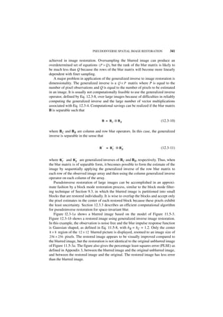
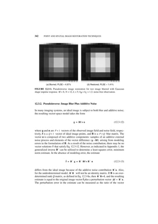
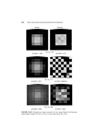
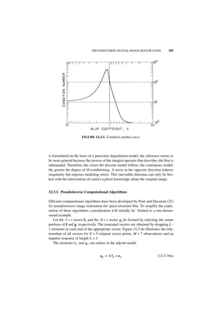
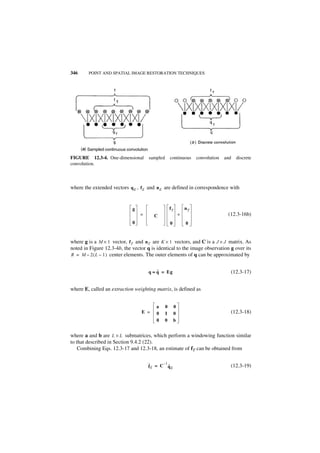
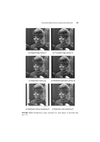
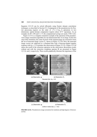
![SVD PSEUDOINVERSE SPATIAL IMAGE RESTORATION 349
extraction operation. Without weighting, errors at the observation boundary
completely destroy the estimate in the boundary region, but with weighting the
restoration is subjectively satisfying, and the restoration error is significantly
reduced. Figure 12.3-6 shows simulation results for the experiment of Figure 12.3-5
when the degree of blur is increased by setting bR = 2.0. The higher degree of blur
greatly increases the ill-conditioning of the blur matrix, and the residual error in
formation of the modified observation after weighting leads to the disappointing
estimate of Figure 12.3-6b. Figure 12.3-6c and d illustrate the restoration improve-
ment obtained with the pseudoinverse algorithm for horizontal image motion blur.
In this example, the blur impulse response is constant, and the corresponding blur
matrix is better conditioned than the blur matrix for Gaussian image blur.
12.4. SVD PSEUDOINVERSE SPATIAL IMAGE RESTORATION
In Appendix 1 it is shown that any matrix can be decomposed into a series of eigen-
matrices by the technique of singular value decomposition. For image restoration,
this concept has been extended (26–29) to the eigendecomposition of blur matrices
in the imaging model
g = Bf + n (12.4-1)
From Eq. A1.2-3, the blur matrix B may be expressed as
1⁄2 T
B = UΛ
Λ V (12.4-2)
where the P × P matrix U and the Q × Q matrix V are unitary matrices composed of
the eigenvectors of BBT and BTB, respectively and Λ is a P × Q matrix whose diag-
onal terms λ ( i ) contain the eigenvalues of BBT and BTB. As a consequence of the
orthogonality of U and V, it is possible to express the blur matrix in the series form
R
1⁄2
∑ [ λ( i )]
T
B = u i vi (12.4-3)
i=1
where ui and v i are the ith columns of U and V, respectively, and R is the rank of
the matrix B.
From Eq. 12.4-2, because U and V are unitary matrices, the generalized inverse
of B is
R
1⁄2 –1 ⁄ 2
∑ [ λ( i ) ]
– T T
B = VΛ
Λ U = vi ui (12.4-4)
i=1
Figure 12.4-1 shows an example of the SVD decomposition of a blur matrix. The
generalized inverse estimate can then be expressed as](https://image.slidesharecdn.com/digitalimageprocessing-120319064358-phpapp01/85/Digital-image-processing-356-320.jpg)
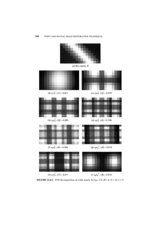
![SVD PSEUDOINVERSE SPATIAL IMAGE RESTORATION 351
ˆ = B– g = VΛ1 ⁄ 2 U T g
f Λ (12.4-5a)
or, equivalently,
R R
ˆ = –1 ⁄ 2 –1 ⁄ 2
∑ ∑ [λ(i)]
T T
f [λ(i )] vi ui g = [ u i g ]v i (12.4-5b)
i=1 i=1
T
recognizing the fact that the inner product u i g is a scalar. Equation 12.4-5 provides
the basis for sequential estimation; the kth estimate of f in a sequence of estimates is
equal to
ˆ = ˆ –1 ⁄ 2 T
fk fk – 1 + [ λ ( k ) ] [ u k g ]v k (12.4-6)
One of the principal advantages of the sequential formulation is that problems of ill-
conditioning generally occur only for higher-order singular values. Thus, it is possi-
ble interactively to terminate the expansion before numerical problems occur.
Figure 12.4-2 shows an example of sequential SVD restoration for the underde-
termined model example of Figure 11.5-3 with a poorly conditioned Gaussian blur
matrix. A one-step pseudoinverse would have resulted in the final image estimate
that is totally overwhelmed by numerical errors. The sixth step, which is the best
subjective restoration, offers a considerable improvement over the blurred original,
but the lowest least-squares error occurs for three singular values.
The major limitation of the SVD image restoration method formulation in Eqs.
12.4-5 and 12.4-6 is computational. The eigenvectors ui and v i must first be deter-
mined for the matrix BBT and BTB. Then the vector computations of Eq 12.4-5 or
12.4-6 must be performed. Even if B is direct-product separable, permitting separa-
ble row and column SVD pseudoinversion, the computational task is staggering in
the general case.
The pseudoinverse computational algorithm described in the preceding section
can be adapted for SVD image restoration in the special case of space-invariant blur
(23). From the adjoint model of Eq. 12.3-16 given by
q E = Cf E + n E (12.4-7)
the circulant matrix C can be expanded in SVD form as
1⁄2 T
C = X∆
∆ Y∗ (12.4-8)
where X and Y are unitary matrices defined by](https://image.slidesharecdn.com/digitalimageprocessing-120319064358-phpapp01/85/Digital-image-processing-358-320.jpg)
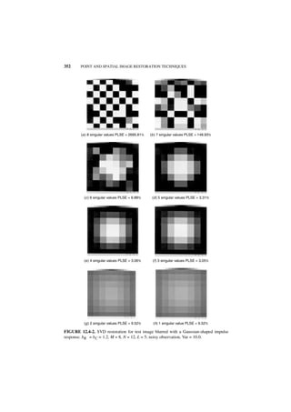
![SVD PSEUDOINVERSE SPATIAL IMAGE RESTORATION 353
T T
X [ CC ]X∗ = ∆ (12.4-9a)
T T
Y [ C C ]Y∗ = ∆ (12.4-9b)
Because C is circulant, CCT is also circulant. Therefore X and Y must be equivalent
–1
to the Fourier transform matrix A or A because the Fourier matrix produces a
diagonalization of a circulant matrix. For purposes of standardization, let
–1
X = Y = A . As a consequence, the eigenvectors x i = y i , which are rows of X
and Y, are actually the complex exponential basis functions
2πi
x k ( j ) = exp ------- ( k – 1 ) ( j – 1 )
* - (12.4-10)
J
of a Fourier transform for 1 ≤ j, k ≤ J . Furthermore,
T
∆ = C C∗ (12.4-11)
where C is the Fourier domain circular area convolution matrix. Then, in correspon-
dence with Eq. 12.4-5
ˆ –1 –1 ⁄ 2
fE = A Λ ˜
Aq E (12.4-12)
˜
where q E is the modified blurred image observation of Eqs. 12.3-19 and 12.3-20.
Equation 12.4-12 should be recognized as being a Fourier domain pseudoinverse
estimate. Sequential SVD restoration, analogous to the procedure of Eq. 12.4-6, can
–1 ⁄ 2
be obtained by replacing the SVD pseudoinverse matrix ∆ of Eq. 12.4-12 by the
operator
–1 ⁄ 2
[ ∆T ( 1 ) ] 0
· –1 ⁄ 2 ·
[ ∆T( 2 ) ]
· ·
–1 ⁄ 2 …
∆T = · –1 ⁄ 2 · (12.4-13)
[ ∆T ( T ) ]
· ·
0
· ·
…
0 0](https://image.slidesharecdn.com/digitalimageprocessing-120319064358-phpapp01/85/Digital-image-processing-360-320.jpg)
![354 POINT AND SPATIAL IMAGE RESTORATION TECHNIQUES
(a) Blurred observation (b) Restoration, T = 58
(c ) Restoration, T = 60
FIGURE 12.4-3. Sequential SVD pseudoinverse image restoration for horizontal Gaussian
blur, bR = 3.0, L = 23, J = 256.
Complete truncation of the high-frequency terms to avoid ill-conditioning effects
may not be necessary in all situations. As an alternative to truncation, the diagonal
–1 ⁄ 2
zero elements can be replaced by [ ∆T ( T ) ] or perhaps by some sequence that
declines in value as a function of frequency. This concept is actually analogous to
the truncated inverse filtering technique defined by Eq. 12.2-11 for continuous
image fields.
Figure 12.4-3 shows an example of SVD pseudoinverse image restoration for
one-dimensional Gaussian image blur with bR = 3.0. It should be noted that the res-
toration attempt with the standard pseudoinverse shown in Figure 12.3-6b was sub-
ject to severe ill-conditioning errors at a blur spread of bR = 2.0.](https://image.slidesharecdn.com/digitalimageprocessing-120319064358-phpapp01/85/Digital-image-processing-361-320.jpg)
![STATISTICAL ESTIMATION SPATIAL IMAGE RESTORATION 355
12.5. STATISTICAL ESTIMATION SPATIAL IMAGE RESTORATION
A fundamental limitation of pseudoinverse restoration techniques is that observation
noise may lead to severe numerical instability and render the image estimate unus-
able. This problem can be alleviated in some instances by statistical restoration
techniques that incorporate some a priori statistical knowledge of the observation
noise (21).
12.5.1. Regression Spatial Image Restoration
Consider the vector-space model
g = Bf + n (12.5-1)
for a blurred image plus additive noise in which B is a P × Q blur matrix and the
noise is assumed to be zero mean with known covariance matrix Kn. The regression
method seeks to form an estimate
ˆ
f = Wg (12.5-2)
where W is a restoration matrix that minimizes the weighted error measure
ˆ ˆ T –1 ˆ
Θ { f } = [ g – Bf ] K n [ g – Bf ] (12.5-3)
Minimization of the restoration error can be accomplished by the classical method
ˆ ˆ
of setting the partial derivative of Θ { f } with respect to f to zero. In the underdeter-
mined case, for which P < Q , it can be shown (30) that the minimum norm estimate
regression operator is
–1 – –1
W = [K B] K (12.5-4)
where K is a matrix obtained from the spectral factorization
T
K n = KK (12.5-5)
2
of the noise covariance matrix K n. For white noise, K = σ n I, and the regression
operator assumes the form of a rank P generalized inverse for an underdetermined
system as given by Eq. 12.3-8b.](https://image.slidesharecdn.com/digitalimageprocessing-120319064358-phpapp01/85/Digital-image-processing-362-320.jpg)
![356 POINT AND SPATIAL IMAGE RESTORATION TECHNIQUES
12.5.2. Wiener Estimation Spatial Image Restoration
With the regression technique of spatial image restoration, the noise field is modeled
as a sample of a two-dimensional random process with a known mean and covari-
ance function. Wiener estimation techniques assume, in addition, that the ideal
image is also a sample of a two-dimensional random process with known first and
second moments (21,22,31).
Wiener Estimation: General Case. Consider the general discrete model of Figure
12.5-1 in which a Q × 1 image vector f is subject to some unspecified type of point
and spatial degradation resulting in the P × 1 vector of observations g. An estimate
of f is formed by the linear operation
ˆ = Wg + b
f (12.5-6)
where W is a Q × P restoration matrix and b is a Q × 1 bias vector. The objective of
Wiener estimation is to choose W and b to minimize the mean-square restoration
error, which may be defined as
E = E{[f – ˆ] [f – ˆ] }
T
f f (12.5-7a)
or
E = tr { E { [ f – ˆ ] [ f – ˆ ] } }
T
f f (12.5-7b)
Equation 12.5-7a expresses the error in inner-product form as the sum of the squares
of the elements of the error vector [ f – ˆ ], while Eq. 12.5-7b forms the covariance
f
matrix of the error, and then sums together its variance terms (diagonal elements) by
the trace operation. Minimization of Eq. 12.5-7 in either of its forms can
be accomplished by differentiation of E with respect to ˆ . An alternative approach,
f
FIGURE 12.5-1. Wiener estimation for spatial image restoration.](https://image.slidesharecdn.com/digitalimageprocessing-120319064358-phpapp01/85/Digital-image-processing-363-320.jpg)
![STATISTICAL ESTIMATION SPATIAL IMAGE RESTORATION 357
which is of quite general utility, is to employ the orthogonality principle (32, p. 219)
to determine the values of W and b that minimize the mean-square error. In the con-
text of image restoration, the orthogonality principle specifies two necessary and
sufficient conditions for the minimization of the mean-square restoration error:
1. The expected value of the image estimate must equal the expected value of
the image
E{ ˆ} = E{f }
f (12.5-8)
2. The restoration error must be orthogonal to the observation about its mean
E{[f – ˆ][g – E{g }] } = 0
T
f (12.5-9)
From condition 1, one obtains
b = E { f } – WE { g } (12.5-10)
and from condition 2
T
E{[ W + b – f][g – E{g }] } = 0 (12.5-11)
Upon substitution for the bias vector b from Eq. 12.5-10 and simplification, Eq.
12.5-11 yields
–1
W = K fg [ K gg ] (12.5-12)
where K gg is the P × P covariance matrix of the observation vector (assumed nons-
ingular) and K fg is the Q × P cross-covariance matrix between the image and obser-
vation vectors. Thus, the optimal bias vector b and restoration matrix W may be
directly determined in terms of the first and second joint moments of the ideal image
and observation vectors. It should be noted that these solutions apply for nonlinear
and space-variant degradations. Subsequent sections describe applications of
Wiener estimation to specific restoration models.
Wiener Estimation: Image Blur with Additive Noise. For the discrete model for a
blurred image subjective to additive noise given by
g = Bf + n (12.5-13)](https://image.slidesharecdn.com/digitalimageprocessing-120319064358-phpapp01/85/Digital-image-processing-364-320.jpg)
![358 POINT AND SPATIAL IMAGE RESTORATION TECHNIQUES
the Wiener estimator is composed of a bias term
b = E { f } – WE { g } = E { f } – WBE { f } + WE { n } (12.5-14)
and a matrix operator
–1 T T –1
W = K fg [ K gg ] = K f B [ BK f B + K n ] (12.5-15)
2 2
If the ideal image field is assumed uncorrelated, K f = σ f I where σ f represents
the image energy. Equation 12.5-15 then reduces to
2 T 2 T –1
W = σ f B [ σ f BB + K n ] (12.5-16)
2
For a white-noise process with energy σ n , the Wiener filter matrix becomes
2
T T σn
W = B BB + ----- I
- (12.5-17)
2
σ f
2 2
As the ratio of image energy to noise energy ( σ f ⁄ σ n ) approaches infinity, the
Wiener estimator of Eq. 12.5-17 becomes equivalent to the generalized inverse esti-
mator.
Figure 12.5-2 shows restoration examples for the model of Figure 11.5-3 for a
Gaussian-shaped blur function. Wiener restorations of large size images are given in
Figure 12.5-3 using a fast computational algorithm developed by Pratt and Davarian
(22). In the example of Figure 12.5-3a illustrating horizontal image motion blur, the
impulse response is of rectangular shape of length L = 11. The center pixels have
been restored and replaced within the context of the blurred image to show the
visual restoration improvement. The noise level and blur impulse response of the
electron microscope original image of Figure 12.5-3c were estimated directly from
the photographic transparency using techniques to be described in Section 12.7. The
parameters were then utilized to restore the center pixel region, which was then
replaced in the context of the blurred original.
12.6. CONSTRAINED IMAGE RESTORATION
The previously described image restoration techniques have treated images as arrays
of numbers. They have not considered that a restored natural image should be sub-
ject to physical constraints. A restored natural image should be spatially smooth and
strictly positive in amplitude.](https://image.slidesharecdn.com/digitalimageprocessing-120319064358-phpapp01/85/Digital-image-processing-365-320.jpg)
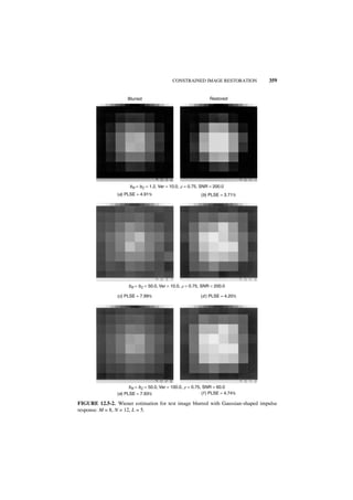
![360 POINT AND SPATIAL IMAGE RESTORATION TECHNIQUES
(a) Observation (b) Restoration
(c) Observation (d ) Restoration
FIGURE 12.5-3. Wiener image restoration.
12.6.1. Smoothing Methods
Smoothing and regularization techniques (33–35) have been used in an attempt to
overcome the ill-conditioning problems associated with image restoration. Basi-
cally, these methods attempt to force smoothness on the solution of a least-squares
error problem.
Two formulations of these methods are considered (21). The first formulation
consists of finding the minimum of ˆ Sf subject to the equality constraint
f ˆ
T
ˆ T ˆ
[ g – Bf ] M [ g – Bf ] = e (12.6-1)
where S is a smoothing matrix, M is an error-weighting matrix, and e denotes a
residual scalar estimation error. The error-weighting matrix is often chosen to be](https://image.slidesharecdn.com/digitalimageprocessing-120319064358-phpapp01/85/Digital-image-processing-367-320.jpg)
![CONSTRAINED IMAGE RESTORATION 361
–1
equal to the inverse of the observation noise covariance matrix, M = K n . The
Lagrangian estimate satisfying Eq. 12.6-1 is (19)
–1 T – 1 T 1 –1 –1
ˆ
f = S B BS B + -- M
- g (12.6-2)
γ
In Eq. 12.6-2, the Lagrangian factor γ is chosen so that Eq. 12.6-1 is satisfied; that
is, the compromise between residual error and smoothness of the estimator is
deemed satisfactory.
Now consider the second formulation, which involves solving an equality-con-
strained least-squares problem by minimizing the left-hand side of Eq. 12.6-1 such
that
ˆT ˆ
f Sf = d (12.6-3)
where the scalar d represents a fixed degree of smoothing. In this case, the optimal
solution for an underdetermined nonsingular system is found to be
ˆ = S –1 B T [ BS – 1 B T + γM– 1 ] –1 g
f (12.6-4)
A comparison of Eqs. 12.6-2 and 12.6-4 reveals that the two inverse problems are
solved by the same expression, the only difference being the Lagrange multipliers,
which are inverses of one another. The smoothing estimates of Eq. 12.6-4 are
closely related to the regression and Wiener estimates derived previously. If γ = 0,
–1
S = I and M = K n where K n is the observation noise covariance matrix, then the
smoothing and regression estimates become equivalent. Substitution of γ = 1,
–1 –1
S = K f and M = K n where K f is the image covariance matrix results in
equivalence to the Wiener estimator. These equivalences account for the relative
smoothness of the estimates obtained with regression and Wiener restoration as
compared to pseudoinverse restoration. A problem that occurs with the smoothing
and regularizing techniques is that even though the variance of a solution can be
calculated, its bias can only be determined as a function of f.
12.6.2. Constrained Restoration Techniques
Equality and inequality constraints have been suggested (21) as a means of improving
restoration performance for ill-conditioned restoration models. Examples of con-
straints include the specification of individual pixel values, of ratios of the values of
some pixels, or the sum of part or all of the pixels, or amplitude limits of pixel values.
Quite often a priori information is available in the form of inequality constraints
involving pixel values. The physics of the image formation process requires that](https://image.slidesharecdn.com/digitalimageprocessing-120319064358-phpapp01/85/Digital-image-processing-368-320.jpg)
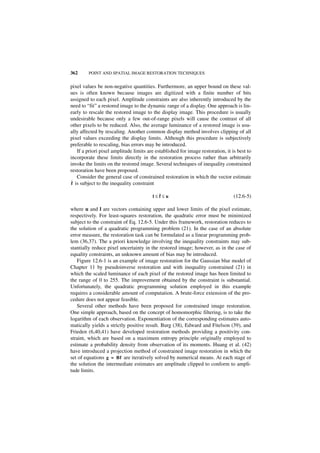
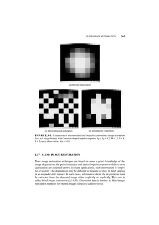

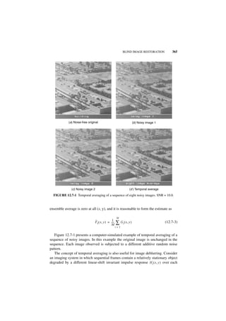
![366 POINT AND SPATIAL IMAGE RESTORATION TECHNIQUES
frame. This type of imaging would be encountered, for example, when photograph-
ing distant objects through a turbulent atmosphere if the object does not move
significantly between frames. By taking a short exposure at each frame, the atmo-
spheric turbulence is “frozen” in space at each frame interval. For this type of
object, the degraded image at the ith frame interval is given by
G i ( x, y ) = F I ( x, y ) ᭺ H i ( x, y )
* (12.7-4)
for i = 1, 2,..., M. The Fourier spectra of the degraded images are then
G i ( ω x, ω y ) = F I ( ω x, ω y )H i ( ω x, ω y ) (12.7-5)
On taking the logarithm of the degraded image spectra
ln { G i ( ω x, ω y ) } = ln { F I ( ω x, ω y ) } + ln { H i ( ω x, ω y ) } (12.7-6)
the spectra of the ideal image and the degradation transfer function are found to sep-
arate additively. It is now possible to apply any of the common methods of statistical
estimation of a signal in the presence of additive noise. If the degradation impulse
responses are uncorrelated between frames, it is worthwhile to form the sum
M M
∑ ln { G i ( ω x, ω y ) } = M ln { F I ( ω x, ω y ) } + ∑ ln { H i ( ω x, ω y ) } (12.7-7)
i=1 i=1
because for large M the latter summation approaches the constant value
M
H M ( ω x, ω y ) = lim ∑ ln { H i ( ω x, ω y ) } (12.7-8)
M → ∞ i = 1
The term H M ( ω x, ω y ) may be viewed as the average logarithm transfer function of
the atmospheric turbulence. An image estimate can be expressed as
M
H M ( ω x, ω y ) 1⁄M
ˆ
F I ( ω x, ω y ) = exp – ----------------------------
M
-
∏ [ G i ( ω x, ω y ) ] (12.7-9)
i=1
An inverse Fourier transform then yields the spatial domain estimate. In any practi-
cal imaging system, Eq. 12.7-4 must be modified by the addition of a noise compo-
nent Ni(x, y). This noise component unfortunately invalidates the separation step of
Eq. 12.7-6, and therefore destroys the remainder of the derivation. One possible
ad hoc solution to this problem would be to perform noise smoothing or filtering on](https://image.slidesharecdn.com/digitalimageprocessing-120319064358-phpapp01/85/Digital-image-processing-373-320.jpg)


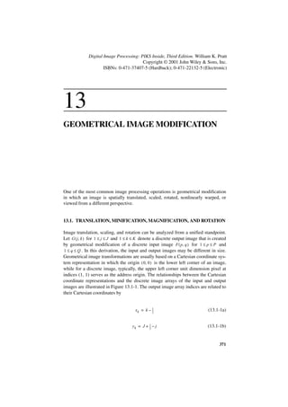


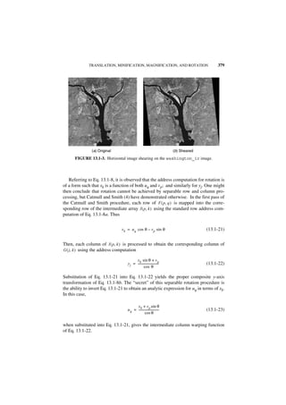
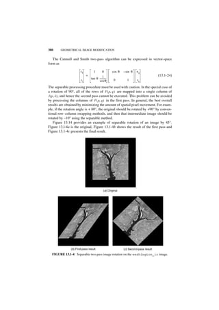
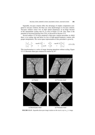
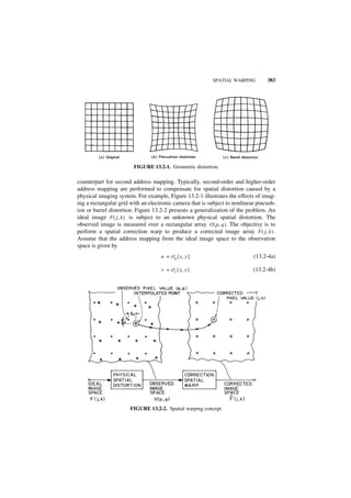
![384 GEOMETRICAL IMAGE MODIFICATION
where Ou { x, y } and O v { x, y } are physical mapping functions. If these mapping
functions are known, then Eq. 13.2-4 can, in principle, be inverted to obtain the
proper corrective spatial warp mapping. If the physical mapping functions are not
known, Eq. 13.2-3 can be considered as an estimate of the physical mapping func-
tions based on the weighting coefficients ( a i, b i ) . These polynomial weighting coef-
ficients are normally chosen to minimize the mean-square error between a set of
observation coordinates ( u m, v m ) and the polynomial estimates ( u, v ) for a set
( 1 ≤ m ≤ M ) of known data points ( x m, y m ) called control points. It is convenient to
arrange the observation space coordinates into the vectors
T
u = [ u 1, u 2, …, u M ] (13.2-5a)
T
v = [ v 1, v 2, …, v M ] (13.2-5b)
Similarly, let the second-order polynomial coefficients be expressed in vector form as
T
a = [ a 0, a 1, …, a 5 ] (13.2-6a)
T
b = [ b 0, b 1, …, b 5 ] (13.2-6b)
The mean-square estimation error can be expressed in the compact form
T T
E = ( u – Aa ) ( u – Aa ) + ( v – Ab ) ( v – Ab ) (13.2-7)
where
2 2
1 x1 y1 x1 x1 y1 y1
2 2
1 x2 y2 x2 x2 y2 y2
A = (13.2-8)
2 2
1 xM yM xM xM yM yM
From Appendix 1, it has been determined that the error will be minimum if
–
a = A u (13.2-9a)
–
b = A v (13.2-9b)
where A– is the generalized inverse of A. If the number of control points is chosen
greater than the number of polynomial coefficients, then
– T –1
A = [A A] A (13.2-10)](https://image.slidesharecdn.com/digitalimageprocessing-120319064358-phpapp01/85/Digital-image-processing-390-320.jpg)
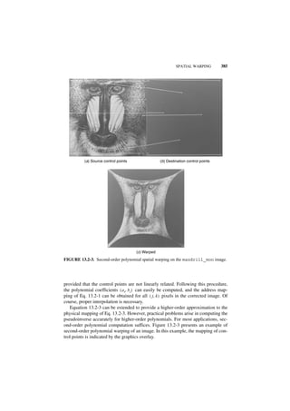
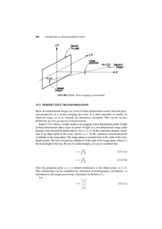

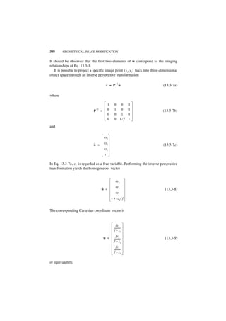
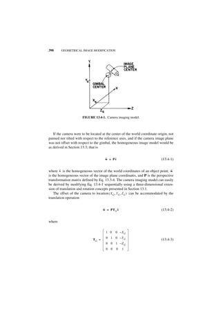
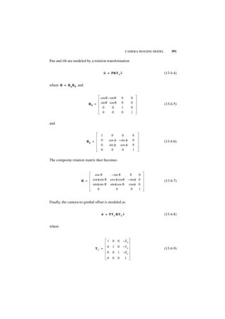
![392 GEOMETRICAL IMAGE MODIFICATION
Equation 13.4-8 is the final result giving the complete camera imaging model trans-
formation between an object and an image point. The explicit relationship between
an object point ( X, Y, Z ) and its image plane projection ( x, y ) can be obtained by
performing the matrix multiplications analytically and then forming the Cartesian
˜
coordinates by dividing the first two components of w by the fourth. Upon perform-
ing these operations, one obtains
f [ ( X – X G ) cos θ – ( Y – Y G ) sin θ – X 0 ]
x = --------------------------------------------------------------------------------------------------------------------------------------------------------------------
- (13.4-10a)
– ( X – X G ) sin θ sin φ – ( Y – Y G ) cos θ sin φ – ( Z – Z G ) cos φ + Z 0 + f
f [ ( X – XG ) sin θ cos φ + ( Y – Y G ) cos θ cos φ – ( Z – Z G ) sin φ – Y 0 ]
y = ------------------------------------------------------------------------------------------------------------------------------------------------------------------
- (13.4-10b)
– ( X – X G ) sin θ sin φ – ( Y – Y G ) cosθ sin φ – ( Z – Z G ) cos φ + Z 0 + f
Equation 13.4-10 can be used to predict the spatial extent of the image of a physical
scene on an imaging sensor.
Another important application of the camera imaging model is to form an image
by postprocessing such that the image appears to have been taken by a camera at a
˜ ˜
different physical perspective. Suppose that two images defined by w 1 and w 2 are
formed by taking two views of the same object with the same camera. The resulting
camera model relationships are then
˜ ˜
w 1 = PT C R 1 T G1 v (13.4-11a)
˜ ˜
w 2 = PT C R 2 T G2 v (13.4-11b)
Because the camera is identical for the two images, the matrices P and TC are
invariant in Eq. 13.4-11. It is now possible to perform an inverse computation of Eq.
13.4-11b to obtain
–1 –1 –1 –1
˜ ˜
v = [ TG1 ] [ R 1 ] [ TC ] [ P ] w 1 (13.4-12)
and by substitution into Eq. 13.4-11b, it is possible to relate the image plane coordi-
nates of the image of the second view to that obtained in the first view. Thus
–1 –1 –1 –1
˜ ˜
w 2 = PT C R 2 TG2 [ T G1 ] [ R 1 ] [ T C ] [ P ] w 1 (13.4-13)
As a consequence, an artificial image of the second view can be generated by per-
forming the matrix multiplications of Eq. 13.4-13 mathematically on the physical
image of the first view. Does this always work? No, there are limitations. First, if
some portion of a physical scene were not “seen” by the physical camera, perhaps it](https://image.slidesharecdn.com/digitalimageprocessing-120319064358-phpapp01/85/Digital-image-processing-398-320.jpg)
![GEOMETRICAL IMAGE RESAMPLING 393
was occluded by structures within the scene, then no amount of processing will rec-
reate the missing data. Second, the processed image may suffer severe degradations
resulting from undersampling if the two camera aspects are radically different. Nev-
ertheless, this technique has valuable applications.
13.5. GEOMETRICAL IMAGE RESAMPLING
As noted in the preceding sections of this chapter, the reverse address computation
process usually results in an address result lying between known pixel values of an
input image. Thus it is necessary to estimate the unknown pixel amplitude from its
known neighbors. This process is related to the image reconstruction task, as
described in Chapter 4, in which a space-continuous display is generated from an
array of image samples. However, the geometrical resampling process is usually not
spatially regular. Furthermore, the process is discrete to discrete; only one output
pixel is produced for each input address.
In this section, consideration is given to the general geometrical resampling
process in which output pixels are estimated by interpolation of input pixels. The
special, but common case, of image magnification by an integer zooming factor is
also discussed. In this case, it is possible to perform pixel estimation by convolution.
13.5.1. Interpolation Methods
The simplest form of resampling interpolation is to choose the amplitude of an out-
put image pixel to be the amplitude of the input pixel nearest to the reverse address.
This process, called nearest-neighbor interpolation, can result in a spatial offset
error by as much as 1 ⁄ 2 pixel units. The resampling interpolation error can be
significantly reduced by utilizing all four nearest neighbors in the interpolation. A
common approach, called bilinear interpolation, is to interpolate linearly along each
row of an image and then interpolate that result linearly in the columnar direction.
Figure 13.5-1 illustrates the process. The estimated pixel is easily found to be
F ( p′, q′ ) = ( 1 – a ) [ ( 1 – b )F ( p, q ) + bF ( p, q + 1 ) ]
+ a [ ( 1 – b )F ( p + 1, q ) + bF ( p + 1, q + 1 ) ] (13.5-1)
Although the horizontal and vertical interpolation operations are each linear, in gen-
eral, their sequential application results in a nonlinear surface fit between the four
neighboring pixels.
The expression for bilinear interpolation of Eq. 13.5-1 can be generalized for any
interpolation function R { x } that is zero-valued outside the range of ± 1 sample
spacing. With this generalization, interpolation can be considered as the summing of
four weighted interpolation functions as given by](https://image.slidesharecdn.com/digitalimageprocessing-120319064358-phpapp01/85/Digital-image-processing-399-320.jpg)
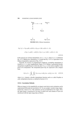
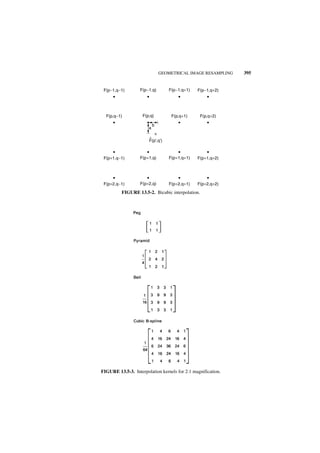
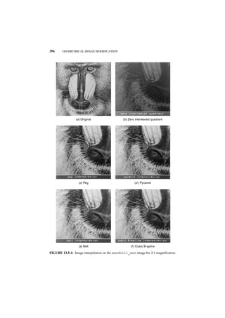


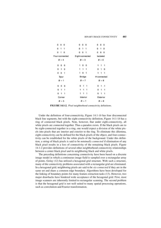

![BINARY IMAGE HIT OR MISS TRANSFORMATIONS 405
FIGURE 14.2-1. Look-up table flowchart for binary unconditional operations.
Several other 3 × 3 hit-or-miss operators are described in the following subsec-
tions.
14.2.1. Additive Operators
Additive hit-or-miss morphological operators cause the center pixel of a 3 × 3 pixel
window to be converted from a logical 0 state to a logical 1 state if the neighboring
pixels meet certain predetermined conditions. The basic operators are now defined.
Interior Fill. Create a black pixel if all four-connected neighbor pixels are black.
G ( j, k ) = X ∪ [ X 0 ∩ X 2 ∩ X 4 ∩ X 6 ] (14.2-2)
Diagonal Fill. Create a black pixel if creation eliminates the eight-connectivity of
the background.
G ( j, k ) = X ∪ [ P 1 ∪ P 2 ∪ P 3 ∪ P 4 ] (14.2-3a)](https://image.slidesharecdn.com/digitalimageprocessing-120319064358-phpapp01/85/Digital-image-processing-410-320.jpg)
![406 MORPHOLOGICAL IMAGE PROCESSING
where
P 1 = X ∩ X0 ∩ X 1 ∩ X 2 (14.2-3b)
P 2 = X ∩ X2 ∩ X 3 ∩ X 4 (14.2-3c)
P 3 = X ∩ X4 ∩ X 5 ∩ X 6 (14.2-3d)
P 4 = X ∩ X6 ∩ X 7 ∩ X 0 (14.2-3e)
In Eq. 14.2-3, the overbar denotes the logical complement of a variable.
Bridge. Create a black pixel if creation results in connectivity of previously uncon-
nected neighboring black pixels.
G ( j, k ) = X ∪ [ P 1 ∪ P 2 ∪ … ∪ P 6 ] (14.2-4a)
where
P 1 = X 2 ∩ X6 ∩ [ X3 ∪ X 4 ∪ X 5 ] ∩ [ X 0 ∪ X 1 ∪ X7 ] ∩ PQ (14.2-4b)
P 2 = X 0 ∩ X4 ∩ [ X1 ∪ X 2 ∪ X 3 ] ∩ [ X 5 ∪ X 6 ∪ X7 ] ∩ PQ (14.2-4c)
P 3 = X 0 ∩ X6 ∩ X7 ∩ [ X 2 ∪ X 3 ∪ X 4 ] (14.2-4d)
P 4 = X 0 ∩ X2 ∩ X1 ∩ [ X 4 ∪ X 5 ∪ X6 ] (14.2-4e)
P 5 = X2 ∩ X4 ∩ X 3 ∩ [ X 0 ∪ X 6 ∪ X7 ] (14.2-4f)
P 6 = X4 ∩ X6 ∩ X 5 ∩ [ X 0 ∪ X 1 ∪ X2 ] (14.2-4g)
and
P Q = L 1 ∪ L2 ∪ L 3 ∪ L 4 (14.2-4h)
L1 = X ∩ X 0 ∩ X1 ∩ X 2 ∩ X 3 ∩ X4 ∩ X5 ∩ X 6 ∩ X 7 (14.2-4i)
L2 = X ∩ X0 ∩ X 1 ∩ X2 ∩ X 3 ∩ X 4 ∩ X5 ∩ X 6 ∩ X 7 (14.2-4j)
L3 = X ∩ X0 ∩ X 1 ∩ X2 ∩ X 3 ∩ X 4 ∩ X5 ∩ X 6 ∩ X 7 (14.2-4k)
L 4 = X ∩ X0 ∩ X 1 ∩ X 2 ∩ X3 ∩ X 4 ∩ X 5 ∩ X6 ∩ X 7 (14.2-4l)](https://image.slidesharecdn.com/digitalimageprocessing-120319064358-phpapp01/85/Digital-image-processing-411-320.jpg)

![408 MORPHOLOGICAL IMAGE PROCESSING
(a) Original
(b) One iteration (c) Three iterations
FIGURE 14.2-2. Dilation of a binary image.
14.2.2. Subtractive Operators
Subtractive hit-or-miss morphological operators cause the center pixel of a 3 × 3
window to be converted from black to white if its neighboring pixels meet predeter-
mined conditions. The basic subtractive operators are defined below.
Isolated Pixel Remove. Erase a black pixel with eight white neighbors.
G ( j, k ) = X ∩ [ X 0 ∪ X 1 ∪ … ∪ X 7 ] (14.2-6)
Spur Remove. Erase a black pixel with a single eight-connected neighbor.](https://image.slidesharecdn.com/digitalimageprocessing-120319064358-phpapp01/85/Digital-image-processing-413-320.jpg)
![BINARY IMAGE HIT OR MISS TRANSFORMATIONS 409
FIGURE 14.2-3. Fattening of a binary image.
The following is one of four qualifying patterns:
0 0 0
0 1 0
1 0 0
Interior Pixel Remove. Erase a black pixel if all four-connected neighbors are
black.
G ( j, k ) = X ∩ [ X 0 ∪ X 2 ∪ X 4 ∪ X 6 ] (14.2-7)
There are 16 qualifying patterns.
H-Break. Erase a black pixel that is H-connected.
There are two qualifying patterns.
1 1 1 1 0 1
0 1 0 1 1 1
1 1 1 1 0 1
Eight-Neighbor Erode. Erase a black pixel if at least one eight-connected neighbor
pixel is white.
G ( j, k ) = X ∩ X 0 ∩ … ∩ X 7 (14.2-8)](https://image.slidesharecdn.com/digitalimageprocessing-120319064358-phpapp01/85/Digital-image-processing-414-320.jpg)

![BINARY IMAGE SHRINKING, THINNING, SKELETONIZING, AND THICKENING 411
14.3. BINARY IMAGE SHRINKING, THINNING, SKELETONIZING, AND
THICKENING
Shrinking, thinning, skeletonizing, and thickening are forms of conditional erosion
in which the erosion process is controlled to prevent total erasure and to ensure con-
nectivity.
14.3.1. Binary Image Shrinking
The following is a definition of shrinking:
Shrink. Erase black pixels such that an object without holes erodes to a single pixel
at or near its center of mass, and an object with holes erodes to a connected ring
lying midway between each hole and its nearest outer boundary.
A 3 × 3 pixel object will be shrunk to a single pixel at its center. A 2 × 2 pixel
object will be arbitrarily shrunk, by definition, to a single pixel at its lower right corner.
It is not possible to perform shrinking using single-stage 3 × 3 pixel hit-or-miss
transforms of the type described in the previous section. The 3 × 3 window does not
provide enough information to prevent total erasure and to ensure connectivity. A
5 × 5 hit-or-miss transform could provide sufficient information to perform proper
shrinking. But such an approach would result in excessive computational complex-
ity (i.e., 225 possible patterns to be examined!). References 15 and 16 describe two-
stage shrinking and thinning algorithms that perform a conditional marking of pixels
for erasure in a first stage, and then examine neighboring marked pixels in a second
stage to determine which ones can be unconditionally erased without total erasure or
loss of connectivity. The following algorithm developed by Pratt and Kabir (17) is a
pipeline processor version of the conditional marking scheme.
In the algorithm, two concatenated 3 × 3 hit-or-miss transformations are per-
formed to obtain indirect information about pixel patterns within a 5 × 5 window.
Figure 14.3-1 is a flowchart for the look-up table implementation of this algorithm.
In the first stage, the states of nine neighboring pixels are gathered together by a
pixel stacker, and a following look-up table generates a conditional mark M for pos-
sible erasures. Table 14.3-1 lists all patterns, as indicated by the letter S in the table
column, which will be conditionally marked for erasure. In the second stage of the
algorithm, the center pixel X and the conditional marks in a 3 × 3 neighborhood cen-
tered about X are examined to create an output pixel. The shrinking operation can be
expressed logically as
G ( j, k ) = X ∩ [ M ∪ P ( M, M 0, …, M 7 ) ] (14.3-1)
where P ( M, M 0, …, M 7 ) is an erasure inhibiting logical variable, as defined in Table
14.3-2. The first four patterns of the table prevent strokes of single pixel width from
being totally erased. The remaining patterns inhibit erasure that would break object
connectivity. There are a total of 157 inhibiting patterns. This two-stage process
must be performed iteratively until there are no further erasures.](https://image.slidesharecdn.com/digitalimageprocessing-120319064358-phpapp01/85/Digital-image-processing-416-320.jpg)
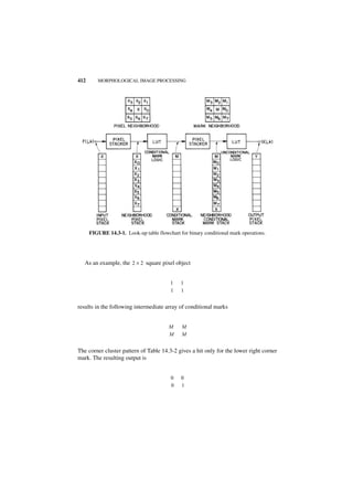
![BINARY IMAGE SHRINKING, THINNING, SKELETONIZING, AND THICKENING 413
TABLE 14.3-1. Shrink, Thin, and Skeletonize Conditional Mark Patterns [M = 1 if hit]
Table Bond Pattern
0 0 1 1 0 0 0 0 0 0 0 0
S 1 0 1 0 0 1 0 0 1 0 0 1 0
0 0 0 0 0 0 1 0 0 0 0 1
0 0 0 0 1 0 0 0 0 0 0 0
S 2 0 1 1 0 1 0 1 1 0 0 1 0
0 0 0 0 0 0 0 0 0 0 1 0
0 0 1 0 1 1 1 1 0 1 0 0 0 0 0 0 0 0 0 0 0 0 0 0
S 3 0 1 1 0 1 0 0 1 0 1 1 0 1 1 0 0 1 0 0 1 0 0 1 1
0 0 0 0 0 0 0 0 0 0 0 0 1 0 0 1 1 0 0 1 1 0 0 1
0 1 0 0 1 0 0 0 0 0 0 0
TK 4 0 1 1 1 1 0 1 1 0 0 1 1
0 0 0 0 0 0 0 1 0 0 1 0
0 0 1 1 1 1 1 0 0 0 0 0
STK 4 0 1 1 0 1 0 1 1 0 0 1 0
0 0 1 0 0 0 1 0 0 1 1 1
1 1 0 0 1 0 0 1 1 0 0 1
ST 5 0 1 1 0 1 1 1 1 0 0 1 1
0 0 0 0 0 1 0 0 0 0 1 0
0 1 1 1 1 0 0 0 0 0 0 0
ST 5 0 1 1 1 1 0 1 1 0 0 1 1
0 0 0 0 0 0 1 1 0 0 1 1
1 1 0 0 1 1
ST 6 0 1 1 1 1 0
0 0 1 1 0 0
1 1 1 0 1 1 1 1 1 1 1 0 1 0 0 0 0 0 0 0 0 0 0 1
STK 6 0 1 1 0 1 1 1 1 0 1 1 0 1 1 0 1 1 0 0 1 1 0 1 1
0 0 0 0 0 1 0 0 0 1 0 0 1 1 0 1 1 1 1 1 1 0 1 1
(Continued)](https://image.slidesharecdn.com/digitalimageprocessing-120319064358-phpapp01/85/Digital-image-processing-418-320.jpg)

![BINARY IMAGE SHRINKING, THINNING, SKELETONIZING, AND THICKENING 415
TABLE 14.3-2. Shrink and Thin Unconditional Mark Patterns
[P(M, M0, M1, M2, M3, M4, M5, M6, M7) = 1 if hit] a
Pattern
Spur Single 4-connection
0 0 M M0 0 0 0 0 0 0 0
0 M0 0 M0 0 M0 0 MM
0 0 0 0 0 0 0 M0 0 0 0
L Cluster (thin only)
0 0 M 0 MM MM0 M0 0 0 0 0 0 0 0 0 0 0 0 0 0
0 MM 0 M0 0 M0 MM0 MM0 0 M0 0 M0 0 MM
0 0 0 0 0 0 0 0 0 0 0 0 M0 0 MM0 0 MM 0 0 M
4-Connected offset
0 MM MM0 0 M0 0 0 M
MM0 0 MM 0 MM 0 MM
0 0 0 0 0 0 0 0 M 0 M0
Spur corner cluster
0 A M MB 0 0 0 M M0 0
0 MB A M0 A M0 0 MB
M0 0 0 0 M MB 0 0 AM
Corner cluster
MMD
MMD
DDD
Tee branch
D M0 0 MD 0 0 D D0 0 D MD 0 M0 0 M0 D MD
MMM MMM MMM MMM MM0 MM0 0 MM 0 MM
D0 0 0 0 D 0 MD D M0 0 M0 D MD D MD 0 M0
Vee branch
MD M MD C CBA A DM
D MD D MB D MD B MD
A B C MD A MD M CDM
Diagonal branch
D M0 0 MD D0 M M0 D
0 MM MM0 MM0 0 MM
M0 D D 0 M 0 MD D M0
a
A∪B∪C = 1 D = 0∪1 A ∪ B = 1.](https://image.slidesharecdn.com/digitalimageprocessing-120319064358-phpapp01/85/Digital-image-processing-420-320.jpg)
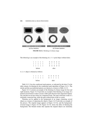

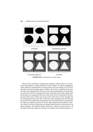
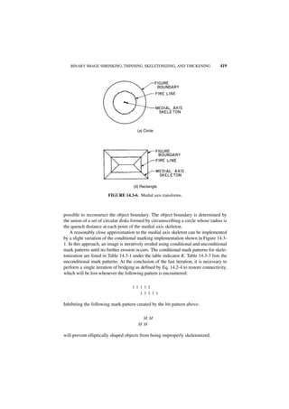
![420 MORPHOLOGICAL IMAGE PROCESSING
TABLE 14.3-3. Skeletonize Unconditional Mark Patterns
[P(M, M0 , M1 , M2, M3, M4, M5, M6 , M7) = 1 if hit]a
Pattern
Spur
0 0 0 0 0 0 0 0 M M 0 0
0 M 0 0 M 0 0 M 0 0 M 0
0 0 M M 0 0 0 0 0 0 0 0
Single 4-connection
0 0 0 0 0 0 0 0 0 0 M 0
0 M 0 0 M M M M 0 0 M 0
0 M 0 0 0 0 0 0 0 0 0 0
L corner
0 M 0 0 M 0 0 0 0 0 0 0
0 M M M M 0 0 M M M M 0
0 0 0 0 0 0 0 M 0 0 M 0
Corner cluster
D M M D D D M M D D D D
D M M M M D M M D D M M
D D D M M D D D D D M M
Tee branch
D M D D M D D D D D M D
M M M M M D M M M D M M
D 0 0 D M D D M D D M D
Vee branch
M D M M D C C B A A D M
D M D D M B D M D B M D
A B C M D A M D M C D M
Digonal branch
D M 0 0 M D D 0 M M 0 D
0 M M M M 0 M M 0 0 M M
M 0 D D 0 M 0 M D D M 0
a
A∪B∪C = 1 D = 0 ∪ 1.](https://image.slidesharecdn.com/digitalimageprocessing-120319064358-phpapp01/85/Digital-image-processing-425-320.jpg)


![426 MORPHOLOGICAL IMAGE PROCESSING
and where Q = ( L – 1 ) ⁄ 2 . Equation 14.4-6 applies for S ≤ j, k ≤ N – Q and
G ( j, k ) = 0 elsewhere. The Minkowski addition definition of generalized erosion
given in Eq. 14.4-2 can be modified to provide a centered result by taking the trans-
lations about the center of the structuring element. In the following discussion, only
the centered definitions of generalized dilation will be utilized. In the special case
for which L = 3, Eq. 14.4-6 can be expressed explicitly as
( G ( j, k ) ) =
[ H ( 3, 3 ) ∩ F ( j – 1, k – 1 ) ] ∪ [ H ( 3, 2 ) ∩ F ( j – 1, k ) ] ∪ [ H ( 3, 1 ) ∩ F ( j – 1, K + 1 ) ]
∪ [ H ( 2, 3 ) ∩ F ( j, k – 1 ) ] ∪ [ H ( 2, 2 ) ∩ F ( j, k ) ] ∪ [ H ( 2, 1 ) ∩ F ( j, k + 1 ) ]
∪ [ H ( 1, 3 ) ∩ F ( j + 1, k – 1 ) ] ∪ [ H ( 1, 2 ) ∩ F ( j + 1, k ) ] ∪ [ H ( 1, 1 ) ∩ F ( j + 1, k + 1 ) ]
(14.4-8)
If H ( j, k ) = 1 for 1 ≤ j, k ≤ 3 , then G ( j, k ) , as computed by Eq. 14.4-8, gives the
same result as hit-or-miss dilation, as defined by Eq. 14.2-5.
It is interesting to compare Eqs. 14.4-6 and 14.4-8, which define generalized
dilation, and Eqs. 7.1-14 and 7.1-15, which define convolution. In the generalized
dilation equation, the union operations are analogous to the summation operations of
convolution, while the intersection operation is analogous to point-by-point
multiplication. As with convolution, dilation can be conceived as the scanning and
processing of F ( j, k ) by H ( j, k ) rotated by 180°.
14.4.2. Generalized Erosion
Generalized erosion is expressed symbolically as
G ( j, k ) = F ( j, k ) ᭺ H ( j, k )
– (14.4-9)
where again H ( j, k ) is an odd size L × L structuring element. Serra (3) has adopted,
as his definition for erosion, the dual relationship of Minkowski addition given by
Eq. 14.4-1, which was introduced by Hadwiger (24). By this formulation, general-
ized erosion is defined to be
G ( j, k ) = ∩ ∩ Tr, c { F ( j, k ) } (14.4-10)
( r, c ) ∈ H
The meaning of this relation is that erosion of F ( j, k ) by H ( j, k ) is the intersection of
all translates of F ( j, k ) in which the translation distance is the row and column index
of pixels of H ( j, k ) that are in the logical 1 state. Steinberg et al. (6,25) have adopted
the subtly different formulation](https://image.slidesharecdn.com/digitalimageprocessing-120319064358-phpapp01/85/Digital-image-processing-431-320.jpg)
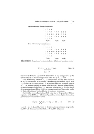
![428 MORPHOLOGICAL IMAGE PROCESSING
G ( j, k ) =
[ H ( 3, 3 ) ∪ F ( j – 1, k – 1 ) ] ∩ [ H ( 3, 2 ) ∪ F ( j – 1, k ) ] ∩ [ H ( 3, 1 ) ∪ F ( j – 1, k + 1 ) ]
∪ [ H ( 2, 3 ) ∪ F ( j, k – 1 ) ] ∩ [ H ( 2, 2 ) ∪ F ( j, k ) ] ∩ [ H ( 2, 1 ) ∪ F ( j, k + 1 ) ]
∩ [ H ( 1, 3 ) ∪ F ( j + 1, k – 1 ) ] ∩ [ H ( 1, 2 ) ∪ F ( j + 1, k ) ] ∩ [ H ( 1, 1 ) ∪ F ( j + 1, k + 1 ) ]
(14.4-13)
If H ( j, k ) = 1 for 1 ≤ j, k ≤ 3 , Eq. 14.4-13 gives the same result as hit-or-miss eight-
neighbor erosion as defined by Eq. 14.2-6. Pratt's definition is the same as the Serra
definition. However, Eq. 14.4-12 can easily be modified by substituting the reflec-
˜
tion H ( j, k ) for H ( j, k ) to provide equivalency with the Steinberg definition.
Unfortunately, the literature utilizes both definitions, which can lead to confusion.
The definition adopted in this book is that of Hadwiger, Serra, and Pratt, because the
FIGURE 14.4-5. Generalized dilation and erosion for a 5 × 5 structuring element.](https://image.slidesharecdn.com/digitalimageprocessing-120319064358-phpapp01/85/Digital-image-processing-433-320.jpg)
![BINARY IMAGE GENERALIZED DILATION AND EROSION 429
defining relationships (Eq. 14.4-1 or 14.4-12) are duals to their counterparts for gen-
eralized dilation (Eq. 14.4-3 or 14.4-6).
Figure 14.4-5 shows examples of generalized dilation and erosion for a symmet-
ric 5 × 5 structuring element.
14.4.3. Properties of Generalized Dilation and Erosion
Consideration is now given to several mathematical properties of generalized
dilation and erosion. Proofs of these properties are found in Reference 25. For nota-
tional simplicity, in this subsection the spatial coordinates of a set are dropped, i.e.,
A( j, k) = A. Dilation is commutative:
A⊕B = B⊕A (14.4-14a)
But in general, erosion is not commutative:
A ᭺B ≠ B᭺A
– – (14.4-14b)
Dilation and erosion are increasing operations in the sense that if A ⊆ B , then
A⊕C⊆B⊕C (14.4-15a)
A᭺ C ⊆ B ᭺ C
– – (14.4-15b)
Dilation and erosion are opposite in effect; dilation of the background of an object
behaves like erosion of the object. This statement can be quantified by the duality
relationship
A᭺ B = A ⊕ B
– (14.4-16)
For the Steinberg definition of erosion, B on the right-hand side of Eq. 14.4-16
˜
should be replaced by its reflection B . Figure 14.4-6 contains an example of the
duality relationship.
The dilation and erosion of the intersection and union of sets obey the following
relations:
[A ∩ B] ⊕ C ⊆ [A ⊕ C] ∩ [B ⊕ C] (14.4-17a)
[ A ∩ B ] ᭺ C = [ A ᭺C ] ∩ [ B ᭺ C ]
– – – (14.4-17b)
[ A ∪ B ] ⊕ C = [ A ⊕ C] ∪ [ B ⊕ C ] (14.4-17c)
[ A ∪ B ] ᭺ C ⊇ [ A ᭺ C ] ∪ [ B ᭺C ]
– – – (14.4-17d)](https://image.slidesharecdn.com/digitalimageprocessing-120319064358-phpapp01/85/Digital-image-processing-434-320.jpg)
![430 MORPHOLOGICAL IMAGE PROCESSING
FIGURE 14.4-6. Duality relationship between dilation and erosion.
The dilation and erosion of a set by the intersection of two other sets satisfy these
containment relations:
A ⊕ [B ∩ C] ⊆ [A ⊕ B] ∩ [A ⊕ C] (14.4-18a)
A᭺ [B ∩ C] ⊇ [A ᭺ B] ∪ [A ᭺ C]
– – – (14.4-18b)
On the other hand, dilation and erosion of a set by the union of a pair of sets are
governed by the equality relations
A ⊕ [B ∪ C] = [A ⊕ B] ∪ [A ⊕ C] (14.4-19a)
A ᭺[ B ∪ C] = [A ᭺B ] ∪ [ A ᭺C]
– – – (14.4-19b)
The following chain rules hold for dilation and erosion.
A ⊕[B ⊕ C] = [ A ⊕ B] ⊕ C (14.4-20a)
A ᭺[B ⊕ C ] = [ A ᭺ B] ᭺ C
– – – (14.4-20b)
14.4.4. Structuring Element Decomposition
Equation 14.4-20 is important because it indicates that if a L × L structuring element
can be expressed as
H ( j, k ) = K 1 ( j, k ) ⊕ … ⊕ Kq ( j, k ) ⊕ … ⊕ K Q ( j, k ) (14.4-21)](https://image.slidesharecdn.com/digitalimageprocessing-120319064358-phpapp01/85/Digital-image-processing-435-320.jpg)


![BINARY IMAGE CLOSE AND OPEN OPERATIONS 433
summed together using the singular-value decomposition/small generating kernel
(SVD/SGK) algorithm, as illustrated by the flowchart of Figure 9.6-2. It is logical to
conjecture as to whether an analog to the SVD/SGK algorithm exists for dilation
and erosion. Equation 14.4-19 suggests that such an algorithm may exist. Figure
14.4-8 illustrates an SSE decomposition of the 5 × 5 ring example based on Eqs.
14.4-19a and 14.4-21. Unfortunately, no systematic method has yet been found to
decompose an arbitrarily large structuring element.
14.5. BINARY IMAGE CLOSE AND OPEN OPERATIONS
Dilation and erosion are often applied to an image in concatenation. Dilation fol-
lowed by erosion is called a close operation. It is expressed symbolically as
G ( j, k ) = F ( j, k ) • H ( j, k ) (14.5-1a)
where H ( j, k ) is a L × L structuring element. In accordance with the Serra formula-
tion of erosion, the close operation is defined as
– ˜
G ( j, k ) = [ F ( j, k ) ⊕ H ( j, k ) ] ᭺ H ( j, k ) (14.5-1b)
where it should be noted that erosion is performed with the reflection of the structur-
ing element. Closing of an image with a compact structuring element without holes
(zeros), such as a square or circle, smooths contours of objects, eliminates small
holes in objects, and fuses short gaps between objects.
An open operation, expressed symbolically as
G ( j, k ) = F ( j, k ) ᭺ H ( j, k ) (14.5-2a)
consists of erosion followed by dilation. It is defined as
– ˜
G ( j, k ) = [ F ( j, k ) ᭺ H ( j, k ) ] ⊕ H ( j, k ) (14.5-2b)
where again, the erosion is with the reflection of the structuring element. Opening of
an image smooths contours of objects, eliminates small objects, and breaks narrow
strokes.
The close operation tends to increase the spatial extent of an object, while the
open operation decreases its spatial extent. In quantitative terms
F ( j, k ) • H ( j, k ) ⊇ F ( j, k ) (14.5-3a)
F ( j, k ) ᭺ H ( j, k ) ⊆ F ( j, k ) (14.5-3b)](https://image.slidesharecdn.com/digitalimageprocessing-120319064358-phpapp01/85/Digital-image-processing-438-320.jpg)
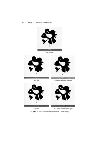
![GRAY SCALE IMAGE MORPHOLOGICAL OPERATIONS 435
It can be shown that the close and open operations are stable in the sense that (25)
[ F ( j, k ) • H ( j, k ) ] • H ( j, k ) = F ( j, k ) • H ( j, k ) (14.5-4a)
[ F ( j, k ) ᭺ H ( j, k ) ] ᭺ H ( j , k ) = F ( j , k ) ᭺H ( j , k ) (14.5-4b)
Also, it can be easily shown that the open and close operations satisfy the following
duality relationship:
F ( j, k ) • H ( j, k ) = F ( j, k ) ᭺H ( j, k ) (14.5-5)
Figure 14.5-1 presents examples of the close and open operations on a binary image.
14.6. GRAY SCALE IMAGE MORPHOLOGICAL OPERATIONS
Morphological concepts can be extended to gray scale images, but the extension
often leads to theoretical issues and to implementation complexities. When applied
to a binary image, dilation and erosion operations cause an image to increase or
decrease in spatial extent, respectively. To generalize these concepts to a gray scale
image, it is assumed that the image contains visually distinct gray scale objects set
against a gray background. Also, it is assumed that the objects and background are
both relatively spatially smooth. Under these conditions, it is reasonable to ask:
Why not just threshold the image and perform binary image morphology? The rea-
son for not taking this approach is that the thresholding operation often introduces
significant error in segmenting objects from the background. This is especially true
when the gray scale image contains shading caused by nonuniform scene illumina-
tion.
14.6.1. Gray Scale Image Dilation and Erosion
Dilation or erosion of an image could, in principle, be accomplished by hit-or-miss
transformations in which the quantized gray scale patterns are examined in a 3 × 3
window and an output pixel is generated for each pattern. This approach is, how-
ever, not computationally feasible. For example, if a look-up table implementation
were to be used, the table would require 2 72 entries for 256-level quantization of
each pixel! The common alternative is to use gray scale extremum operations over a
3 × 3 pixel neighborhoods.
Consider a gray scale image F ( j, k ) quantized to an arbitrary number of gray lev-
els. According to the extremum method of gray scale image dilation, the dilation
operation is defined as
G ( j, k ) = MAX { F ( j, k ), F ( j, k + 1 ), F ( j – 1, k + 1 ), …, F ( j + 1, k + 1 ) } (14.6-1)](https://image.slidesharecdn.com/digitalimageprocessing-120319064358-phpapp01/85/Digital-image-processing-440-320.jpg)
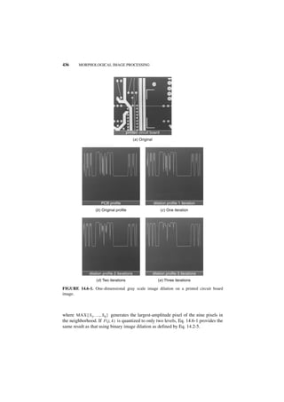

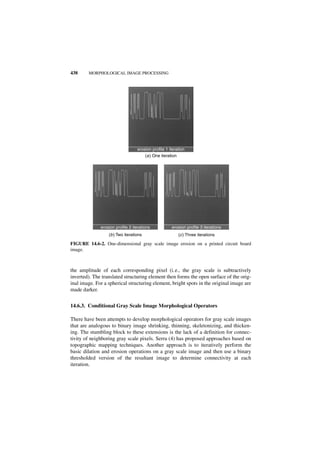
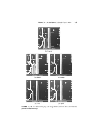


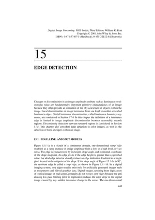
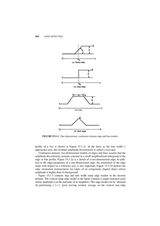
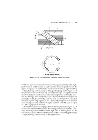
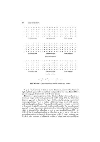
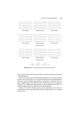

![FIRST-ORDER DERIVATIVE EDGE DETECTION 449
FIGURE 15.1-6. Differential edge, line, and spot detection.
15.2.1. Orthogonal Gradient Generation
An edge in a continuous domain edge segment F ( x, y ) such as the one depicted in
Figure 15.1-2a can be detected by forming the continuous one-dimensional gradient
G ( x, y ) along a line normal to the edge slope, which is at an angle θ with respect to
the horizontal axis. If the gradient is sufficiently large (i.e., above some threshold
value), an edge is deemed present. The gradient along the line normal to the edge
slope can be computed in terms of the derivatives along orthogonal axes according
to the following (1, p. 106)
∂F ( x, y ) ∂F ( x, y )
G ( x, y ) = ------------------- cos θ + ------------------- sin θ
- - (15.2-1)
∂x ∂y
Figure 15.2-1 describes the generation of an edge gradient G ( x, y ) in the discrete
domain in terms of a row gradient G R ( j, k ) and a column gradient G C ( j, k ) . The
spatial gradient amplitude is given by
2 2 1⁄2
G ( j , k ) = [ [ G R ( j, k ) ] + [ G C ( j, k ) ] ] (15.2-2)
For computational efficiency, the gradient amplitude is sometimes approximated by
the magnitude combination
G ( j, k ) = G R ( j, k ) + G C ( j, k ) (15.2-3)
FIGURE 15.2-1. Orthogonal gradient generation.](https://image.slidesharecdn.com/digitalimageprocessing-120319064358-phpapp01/85/Digital-image-processing-453-320.jpg)

![FIRST-ORDER DERIVATIVE EDGE DETECTION 451
(a) Original
(b) Horizontal magnitude (c) Vertical magnitude
FIGURE 15.2-2. Horizontal and vertical differencing gradients of the peppers_mon
image.
Diagonal edge gradients can be obtained by forming running differences of diag-
onal pairs of pixels. This is the basis of the Roberts (2) cross-difference operator,
which is defined in magnitude form as
G ( j, k ) = G 1 ( j, k ) + G 2 ( j, k ) (15.2-6a)
and in square-root form as
2 2 1⁄2
G ( j , k ) = [ [ G 1 ( j, k ) ] + [ G 2 ( j, k ) ] ] (15.2-6b)](https://image.slidesharecdn.com/digitalimageprocessing-120319064358-phpapp01/85/Digital-image-processing-455-320.jpg)
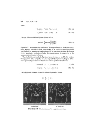
![FIRST-ORDER DERIVATIVE EDGE DETECTION 453
FIGURE 15.2-4. Numbering convention for 3 × 3 edge detection operators.
Although the ramp edge is properly localized, the separated pixel difference gradi-
ent generation method remains highly sensitive to small luminance fluctuations in
the image. This problem can be alleviated by using two-dimensional gradient forma-
tion operators that perform differentiation in one coordinate direction and spatial
averaging in the orthogonal direction simultaneously.
Prewitt (1, p. 108) has introduced a 3 × 3 pixel edge gradient operator described
by the pixel numbering convention of Figure 15.2-4. The Prewitt operator square
root edge gradient is defined as
2 2 1⁄2
G ( j , k ) = [ [ G R ( j, k ) ] + [ G C ( j, k ) ] ] (15.2-9a)
with
1
G R ( j, k ) = ------------ [ ( A 2 + KA 3 + A 4 ) – ( A 0 + KA7 + A6 ) ]
- (15.2-9b)
K+2
1
G C ( j, k ) = ------------ [ ( A0 + KA1 + A2 ) – ( A 6 + KA 5 + A 4 ) ]
- (15.2-9c)
K+2
where K = 1. In this formulation, the row and column gradients are normalized to
provide unit-gain positive and negative weighted averages about a separated edge
position. The Sobel operator edge detector (3, p. 271) differs from the Prewitt edge
detector in that the values of the north, south, east, and west pixels are doubled (i. e.,
K = 2). The motivation for this weighting is to give equal importance to each pixel
in terms of its contribution to the spatial gradient. Frei and Chen (4) have proposed
north, south, east, and west weightings by K = 2 so that the gradient is the same
for horizontal, vertical, and diagonal edges. The edge gradient G ( j, k ) for these three
operators along a row through the single pixel transition vertical ramp edge model
of Figure 15.1-3 is](https://image.slidesharecdn.com/digitalimageprocessing-120319064358-phpapp01/85/Digital-image-processing-457-320.jpg)


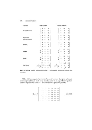
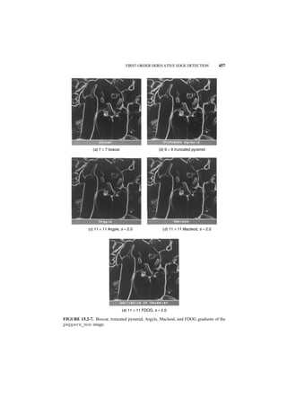
![458 EDGE DETECTION
Argyle (6) and Macleod (7,8) have proposed large neighborhood Gaussian-shaped
weighting functions as a means of noise suppression. Let
2 –1 ⁄ 2 2
g ( x, s ) = [ 2πs ] exp { – 1 ⁄ 2 ( x ⁄ s ) } (15.2-13)
denote a continuous domain Gaussian function with standard deviation s. Utilizing
this notation, the Argyle operator horizontal coordinate impulse response array can
be expressed as a sampled version of the continuous domain impulse response
– 2 g ( x, s )g ( y, t ) for x ≥ 0 (15.2-14a)
H R ( j, k ) =
2g ( x, s )g ( y, t )
for x < 0 (15.2-14b)
where s and t are spread parameters. The vertical impulse response function can be
expressed similarly. The Macleod operator horizontal gradient impulse response
function is given by
H R ( j, k ) = [ g ( x + s, s ) – g ( x – s, s ) ]g ( y, t ) (15.2-15)
The Argyle and Macleod operators, unlike the boxcar operator, give decreasing
importance to pixels far removed from the center of the neighborhood. Figure
15.2-7 provides examples of the Argyle and Macleod gradients.
Extended-size differential gradient operators can be considered to be compound
operators in which a smoothing operation is performed on a noisy image followed
by a differentiation operation. The compound gradient impulse response can be
written as
H ( j, k ) = H G ( j, k ) ᭺ H S ( j, k )
ء (15.2-16)
where H G ( j, k ) is one of the gradient impulse response operators of Figure 15.2-6
and H S ( j, k ) is a low-pass filter impulse response. For example, if H S ( j, k ) is the
3 × 3 Prewitt row gradient operator and H S ( j, k ) = 1 ⁄ 9 , for all ( j, k ) , is a 3 × 3 uni-
form smoothing operator, the resultant 5 × 5 row gradient operator, after normaliza-
tion to unit positive and negative gain, becomes
1 1 0 –1 –1
2 2 0 –2 –2
1
H R = -----
- 3 3 0 –3 –3 (15.2-17)
18
2 2 0 –2 –2
1 1 0 –1 –1](https://image.slidesharecdn.com/digitalimageprocessing-120319064358-phpapp01/85/Digital-image-processing-462-320.jpg)
![FIRST-ORDER DERIVATIVE EDGE DETECTION 459
The decomposition of Eq. 15.2-16 applies in both directions. By applying the SVD/
SGK decomposition of Section 9.6, it is possible, for example, to decompose a 5 × 5
boxcar operator into the sequential convolution of a 3 × 3 smoothing kernel and a
3 × 3 differentiating kernel.
A well-known example of a compound gradient operator is the first derivative of
Gaussian (FDOG) operator, in which Gaussian-shaped smoothing is followed by
differentiation (9). The FDOG continuous domain horizontal impulse response is
– ∂[ g ( x, s )g ( y, t ) ]
H R ( j, k ) = ------------------------------------------
- (15.2-18a)
∂x
which upon differentiation yields
– xg ( x, s )g ( y, t )
HR ( j, k ) = -------------------------------------
- (15.2-18b)
2
s
Figure 15.2-7 presents an example of the FDOG gradient.
All of the differential edge enhancement operators presented previously in this
subsection have been derived heuristically. Canny (9) has taken an analytic
approach to the design of such operators. Canny's development is based on a one-
dimensional continuous domain model of a step edge of amplitude hE plus additive
white Gaussian noise with standard deviation σ n . It is assumed that edge detection
is performed by convolving a one-dimensional continuous domain noisy edge signal
f ( x ) with an antisymmetric impulse response function h ( x ) , which is of zero
amplitude outside the range [ – W, W ] . An edge is marked at the local maximum of
the convolved gradient f ( x ) ᭺ h ( x ). The Canny operator impulse response h ( x ) is
*
chosen to satisfy the following three criteria.
1. Good detection. The amplitude signal-to-noise ratio (SNR) of the gradient is
maximized to obtain a low probability of failure to mark real edge points and a
low probability of falsely marking nonedge points. The SNR for the model is
hE S ( h )
SNR = ----------------
- (15.2-19a)
σn
with
0
∫– W h ( x ) d x
S ( h ) = ---------------------------------- (15.2-19b)
W 2
∫ [ h ( x ) ] dx
–W](https://image.slidesharecdn.com/digitalimageprocessing-120319064358-phpapp01/85/Digital-image-processing-463-320.jpg)
![460 EDGE DETECTION
2. Good localization. Edge points marked by the operator should be as close to
the center of the edge as possible. The localization factor is defined as
hE L ( h )
LOC = ----------------- (15.2-20a)
σn
with
h′ ( 0 )
L ( h ) = -------------------------------------
- (15.2-20b)
W 2
∫ –W
[ h′ ( x ) ] dx
where h′ ( x ) is the derivative of h ( x ) .
3. Single response. There should be only a single response to a true edge. The
distance between peaks of the gradient when only noise is present, denoted as
xm, is set to some fraction k of the operator width factor W. Thus
x m = kW (15.2-21)
Canny has combined these three criteria by maximizing the product S ( h )L ( h ) subject
to the constraint of Eq. 15.2-21. Because of the complexity of the formulation, no
analytic solution has been found, but a variational approach has been developed.
Figure 15.2-8 contains plots of the Canny impulse response functions in terms of xm.
FIGURE 15.2-8. Comparison of Canny and first derivative of Gaussian impulse response
functions.](https://image.slidesharecdn.com/digitalimageprocessing-120319064358-phpapp01/85/Digital-image-processing-464-320.jpg)

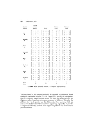
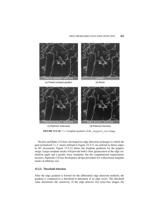


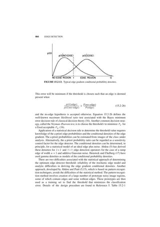

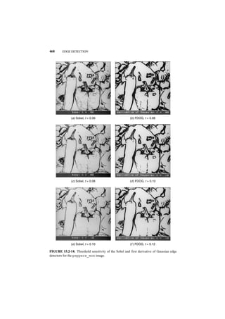
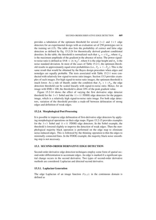
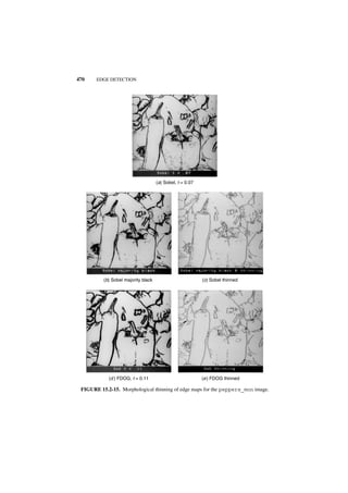
![SECOND-ORDER DERIVATIVE EDGE DETECTION 471
G ( x, y ) = – ∇2{ F ( x, y ) } (15.3-1a)
where, from Eq. 1.2-17, the Laplacian is
2 2
2 ∂ ∂
∇ = + (15.3-1b)
2 2
∂x ∂y
The Laplacian G ( x, y ) is zero if F ( x, y ) is constant or changing linearly in ampli-
tude. If the rate of change of F ( x, y ) is greater than linear, G ( x, y ) exhibits a sign
change at the point of inflection of F ( x, y ). The zero crossing of G ( x, y ) indicates
the presence of an edge. The negative sign in the definition of Eq. 15.3-la is present
so that the zero crossing of G ( x, y ) has a positive slope for an edge whose amplitude
increases from left to right or bottom to top in an image.
Torre and Poggio (18) have investigated the mathematical properties of the
Laplacian of an image function. They have found that if F ( x, y ) meets certain
smoothness constraints, the zero crossings of G ( x, y ) are closed curves.
In the discrete domain, the simplest approximation to the continuous Laplacian is
to compute the difference of slopes along each axis:
G ( j , k ) = [ F ( j, k ) – F ( j, k – 1 ) ] – [ F ( j, k + 1 ) – F ( j, k ) ]
+ [ F ( j, k ) – F ( j + 1, k ) ] – [ F ( j – 1, k ) – F ( j, k ) ] (15.3-2)
This four-neighbor Laplacian (1, p. 111) can be generated by the convolution opera-
tion
G ( j, k ) = F ( j, k ) ᭺ H ( j, k )
ء (15.3-3)
with
0 0 0 0 –1 0
H = –1 2 –1 + 0 2 0 (15.3-4a)
0 0 0 0 –1 0
or
0 –1 0
H = –1 4 – 1 (15.3-4b)
0 –1 0
where the two arrays of Eq. 15.3-4a correspond to the second derivatives along
image rows and columns, respectively, as in the continuous Laplacian of Eq. 15.3-lb.
The four-neighbor Laplacian is often normalized to provide unit-gain averages of the
positive weighted and negative weighted pixels in the 3 × 3 pixel neighborhood. The
gain-normalized four-neighbor Laplacian impulse response is defined by](https://image.slidesharecdn.com/digitalimageprocessing-120319064358-phpapp01/85/Digital-image-processing-475-320.jpg)
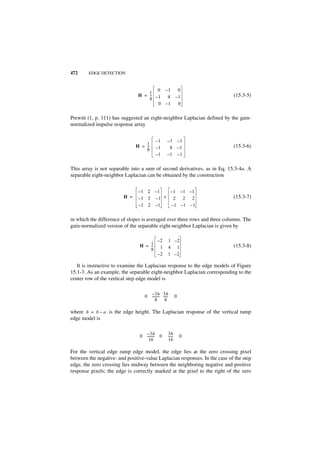

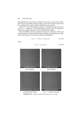


![SECOND-ORDER DERIVATIVE EDGE DETECTION 479
2 2 4
k 1 = a 1 – -- a 4 – -- a 6 + -- a 9
- - - (15.3-19a)
3 3 9
2
k 2 = a 2 – -- a 7
- (15.3-19b)
3
k3 = a3 – 2 a8
--
- (15.3-19c)
3
2
k 4 = a 4 – -- a 9
- (15.3-19d)
3
k5 = a5 (15.3-19e)
2
k 6 = a 6 – -- a 9
- (15.3-19f)
3
k7 = a7 (15.3-19g)
k8 = a8 (15.3-19h)
k9 = a9 (15.3-19i)
The optimum values of the set of weighting coefficients an that minimize the mean-
ˆ
square error between the image data F ( r, c ) and its approximation F ( r, c ) are found
to be (22)
∑ ∑ Pn ( r, c )F ( r, c )
a n = ----------------------------------------------------
- (15.3-20)
2
∑ ∑ [ P n ( r, c ) ]
As a consequence of the linear structure of this equation, the weighting coefficients
An ( j, k ) = a n at each point in the image F ( j, k ) can be computed by convolution of
the image with a set of impulse response arrays. Hence
An ( j, k ) = F ( j, k ) ᭺ H n ( j, k )
ء (15.3-21a)
where
P n ( – j, – k )
H n ( j, k ) = -----------------------------------------
- (15.3-21b)
2
∑ ∑ [ Pn ( r, c ) ]
Figure 15.3-5 contains the nine impulse response arrays corresponding to the 3 × 3
Chebyshev polynomials. The arrays H2 and H3, which are used to determine the
edge angle, are seen from Figure 15.3-5 to be the Prewitt column and row operators,
respectively. The arrays H4 and H6 are second derivative operators along columns](https://image.slidesharecdn.com/digitalimageprocessing-120319064358-phpapp01/85/Digital-image-processing-483-320.jpg)
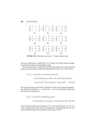
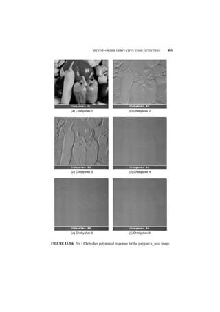
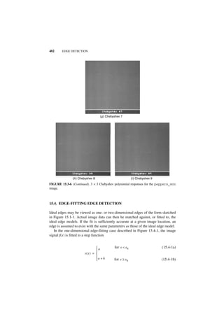
![EDGE-FITTING EDGE DETECTION 483
FIGURE 15.4-1. One- and two-dimensional edge fitting.
An edge is assumed present if the mean-square error
x0 + L 2
E = ∫x 0–L
[ f ( x ) – s ( x ) ] dx (15.4-2)
is below some threshold value. In the two-dimensional formulation, the ideal step
edge is defined as
a for x cos θ + y sin θ < ρ (15.4-3a)
s(x) =
a + h for x cos θ + y sin θ ≥ ρ (15.4-3b)
where θ and ρ jointly specify the polar distance from the center of a circular test
region to the normal point of the edge. The edge-fitting error is
2
E = ∫ ∫ [ F ( x, y ) – S ( x, y ) ] dx dy (15.4-4)
where the integration is over the circle in Figure 15.4-1.](https://image.slidesharecdn.com/digitalimageprocessing-120319064358-phpapp01/85/Digital-image-processing-487-320.jpg)
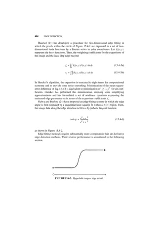

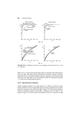
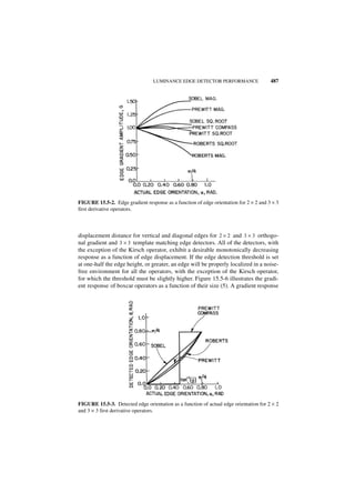
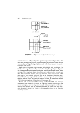
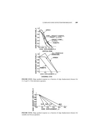
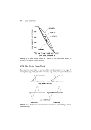
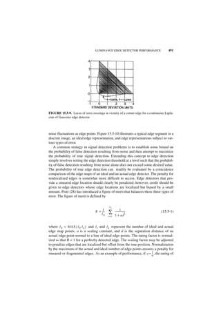
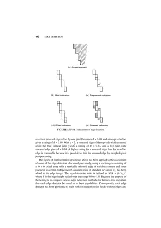
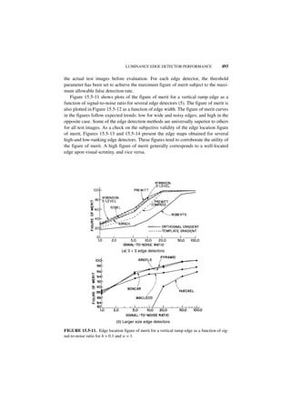
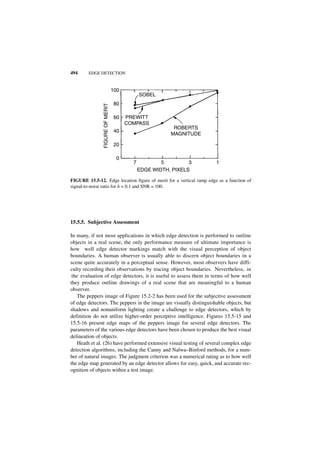
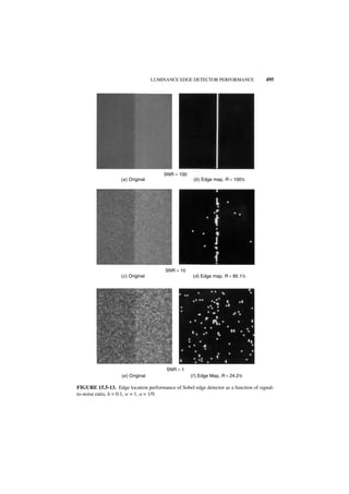
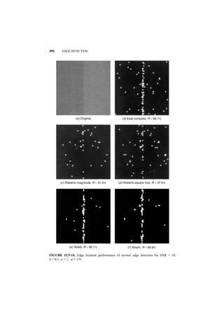
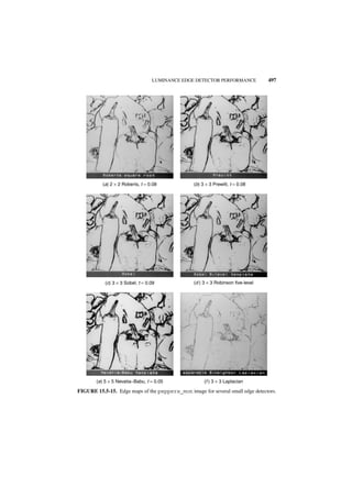
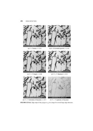
![LINE AND SPOT DETECTION 499
15.6. COLOR EDGE DETECTION
In Chapter 3 it was established that color images may be described quantitatively at
each pixel by a set of three tristimulus values T1, T2, T3, which are proportional to
the amount of red, green, and blue primary lights required to match the pixel color.
The luminance of the color is a weighted sum Y = a 1 T 1 + a 2 T 2 + a 3 T3 of the tris-
timulus values, where the a i are constants that depend on the spectral characteristics
of the primaries.
Several definitions of a color edge have been proposed (29). An edge in a color
image can be said to exist if and only if the luminance field contains an edge. This
definition ignores discontinuities in hue and saturation that occur in regions of con-
stant luminance. Another definition is to judge a color edge present if an edge exists
in any of its constituent tristimulus components. A third definition is based on form-
ing the sum
G ( j, k ) = G 1 ( j, k ) + G 2 ( j, k ) + G 3 ( j, k ) (15.6-1)
of the gradients G i ( j, k ) of the three tristimulus values or some linear or nonlinear
color components. A color edge exists if the gradient exceeds a threshold. Still
another definition is based on the vector sum gradient
2 2 2 1⁄2
G ( j, k ) = [ [ G 1 ( j, k ) ] + [ G 2 ( j, k ) ] + [ G 3 ( j, k ) ] ] (15.6-2)
With the tricomponent definitions of color edges, results are dependent on the
particular color coordinate system chosen for representation. Figure 15.6-1 is a color
photograph of the peppers image and monochrome photographs of its red, green,
and blue components. The YIQ and L*a*b* coordinates are shown in Figure 15.6-2.
Edge maps of the individual RGB components are shown in Figure 15.6-3 for Sobel
edge detection. This figure also shows the logical OR of the RGB edge maps plus
the edge maps of the gradient sum and the vector sum. The RGB gradient vector
sum edge map provides slightly better visual edge delineation than that provided by
the gradient sum edge map; the logical OR edge map tends to produce thick edges
and numerous isolated edge points. Sobel edge maps for the YIQ and the L*a*b*
color components are presented in Figures 15.6-4 and 15.6-5. The YIQ gradient vec-
tor sum edge map gives the best visual edge delineation, but it does not delineate
edges quite as well as the RGB vector sum edge map. Edge detection results for the
L*a*b* coordinate system are quite poor because the a* component is very noise
sensitive.
15.7 LINE AND SPOT DETECTION
A line in an image could be considered to be composed of parallel, closely spaced
edges. Similarly, a spot could be considered to be a closed contour of edges. This](https://image.slidesharecdn.com/digitalimageprocessing-120319064358-phpapp01/85/Digital-image-processing-503-320.jpg)
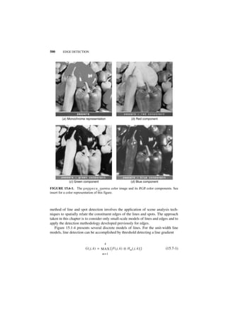
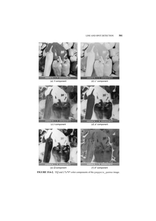
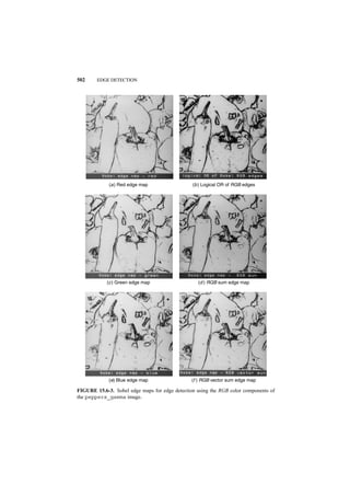
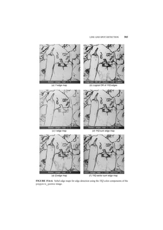
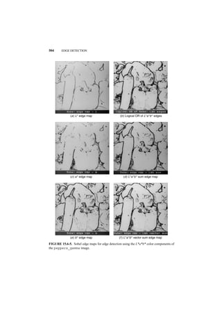
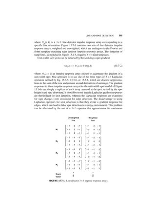
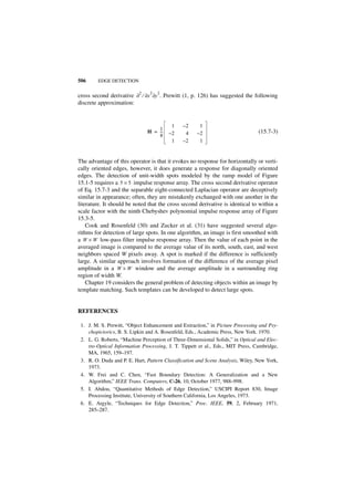


![510 IMAGE FEATURE EXTRACTION
segmentation procedure using a test set of features. Then, the detected segments are
compared to the known segments, and the segmentation error is evaluated. The
problems associated with the prototype performance methods of feature evaluation
are the integrity of the prototype data and the fact that the performance indication is
dependent not only on the quality of the features but also on the classification or seg-
mentation ability of the classifier or segmenter.
The figure-of-merit approach to feature evaluation involves the establishment of
some functional distance measurements between sets of image features such that a
large distance implies a low classification error, and vice versa. Faugeras and Pratt
(5) have utilized the Bhattacharyya distance (3) figure-of-merit for texture feature
evaluation. The method should be extensible for other features as well. The Bhatta-
charyya distance (B-distance for simplicity) is a scalar function of the probability
densities of features of a pair of classes defined as
1⁄2
B ( S 1, S 2 ) = – ln ∫ [ p ( x S 1 )p ( x S 2 ) ] dx (16.1-1)
where x denotes a vector containing individual image feature measurements with
conditional density p ( x S i ) . It can be shown (3) that the B-distance is related mono-
tonically to the Chernoff bound for the probability of classification error using a
Bayes classifier. The bound on the error probability is
1⁄2
P ≤ [ P ( S 1 )P ( S2 ) ] exp { – B ( S 1, S 2 ) } (16.1-2)
where P ( Si ) represents the a priori class probability. For future reference, the Cher-
noff error bound is tabulated in Table 16.1-1 as a function of B-distance for equally
likely feature classes.
For Gaussian densities, the B-distance becomes
1
T Σ1 + Σ2
–1 -- Σ 1 + Σ 2
-
B ( S 1, S 2 ) = 1 ( u 1 – u 2 ) ----------------- ( u 1 – u 2 ) + 1 ln --------------------------------- (16.1-3)
--
- - --
-
2
-
8 2 2
Σ1 1 ⁄ 2 Σ2 1 ⁄ 2
where ui and Σ i represent the feature mean vector and the feature covariance matrix
of the classes, respectively. Calculation of the B-distance for other densities is gener-
ally difficult. Consequently, the B-distance figure of merit is applicable only for
Gaussian-distributed feature data, which fortunately is the common case. In prac-
tice, features to be evaluated by Eq. 16.1-3 are measured in regions whose class has
been determined independently. Sufficient feature measurements need be taken so
that the feature mean vector and covariance can be estimated accurately.](https://image.slidesharecdn.com/digitalimageprocessing-120319064358-phpapp01/85/Digital-image-processing-514-320.jpg)
![AMPLITUDE FEATURES 511
TABLE 16.1-1 Relationship of Bhattacharyya Distance
and Chernoff Error Bound
B ( S 1, S 2 ) Error Bound
1 1.84 × 10⁻¹
2 6.77 × 10⁻²
4 9.16 × 10⁻³
6 1.24 × 10⁻³
8 1.68 × 10⁻⁴
10 2.27 × 10⁻⁵
12 2.07 × 10⁻⁶
16.2. AMPLITUDE FEATURES
The most basic of all image features is some measure of image amplitude in terms of
luminance, tristimulus value, spectral value, or other units. There are many degrees
of freedom in establishing image amplitude features. Image variables such as lumi-
nance or tristimulus values may be utilized directly, or alternatively, some linear,
nonlinear, or perhaps noninvertible transformation can be performed to generate
variables in a new amplitude space. Amplitude measurements may be made at spe-
cific image points, [e.g., the amplitude F ( j, k ) at pixel coordinate ( j, k ) , or over a
neighborhood centered at ( j, k ) ]. For example, the average or mean image amplitude
in a W × W pixel neighborhood is given by
w w
1
M ( j, k ) = ------
W
-
2 ∑ ∑ F ( j + m, k + n ) (16.2-1)
m = –w n = –w
where W = 2w + 1. An advantage of a neighborhood, as opposed to a point measure-
ment, is a diminishing of noise effects because of the averaging process. A disadvan-
tage is that object edges falling within the neighborhood can lead to erroneous
measurements.
The median of pixels within a W × W neighborhood can be used as an alternative
amplitude feature to the mean measurement of Eq. 16.2-1, or as an additional
feature. The median is defined to be that pixel amplitude in the window for which
one-half of the pixels are equal or smaller in amplitude, and one-half are equal or
greater in amplitude. Another useful image amplitude feature is the neighborhood
standard deviation, which can be computed as
w w 1⁄2
1 2
S ( j, k ) = ----
W
- ∑ ∑ [ F ( j + m, k + n ) – M ( j + m, k + n ) ] (16.2-2)
m = –w n = – w](https://image.slidesharecdn.com/digitalimageprocessing-120319064358-phpapp01/85/Digital-image-processing-515-320.jpg)
![512 IMAGE FEATURE EXTRACTION
(a) Original (b) 7 × 7 pyramid mean
(c) 7 × 7 standard deviation (d ) 7 × 7 plus median
FIGURE 16.2-1. Image amplitude features of the washington_ir image.
In the literature, the standard deviation image feature is sometimes called the image
dispersion. Figure 16.2-1 shows an original image and the mean, median, and stan-
dard deviation of the image computed over a small neighborhood.
The mean and standard deviation of Eqs. 16.2-1 and 16.2-2 can be computed
indirectly in terms of the histogram of image pixels within a neighborhood. This
leads to a class of image amplitude histogram features. Referring to Section 5.7, the
first-order probability distribution of the amplitude of a quantized image may be
defined as
P ( b ) = P R [ F ( j, k ) = r b ] (16.2-3)
where r b denotes the quantized amplitude level for 0 ≤ b ≤ L – 1 . The first-order his-
togram estimate of P(b) is simply](https://image.slidesharecdn.com/digitalimageprocessing-120319064358-phpapp01/85/Digital-image-processing-516-320.jpg)
![AMPLITUDE FEATURES 513
N( b)
P ( b ) ≈ -----------
- (16.2-4)
M
where M represents the total number of pixels in a neighborhood window centered
about ( j, k ) , and N ( b ) is the number of pixels of amplitude r b in the same window.
The shape of an image histogram provides many clues as to the character of the
image. For example, a narrowly distributed histogram indicates a low-contrast
image. A bimodal histogram often suggests that the image contains an object with a
narrow amplitude range against a background of differing amplitude. The following
measures have been formulated as quantitative shape descriptions of a first-order
histogram (6).
Mean:
L–1
SM ≡ b = ∑ bP ( b ) (16.2-5)
b=0
Standard deviation:
L–1 1⁄2
2
SD ≡ σb = ∑ (b – b ) P( b) (16.2-6)
b=0
Skewness:
L–1
1 3
S S = -----
σb
-
3 ∑ ( b – b) P(b ) (16.2-7)
b=0
Kurtosis:
L–1
1- 4
S K = -----
4 ∑ ( b – b) P( b ) – 3 (16.2-8)
σb b=0
Energy:
L–1
2
SN = ∑ [P(b )] (16.2-9)
b=0
Entropy:
L–1
SE = – ∑ P ( b ) log 2 { P ( b ) } (16.2-10)
b=0](https://image.slidesharecdn.com/digitalimageprocessing-120319064358-phpapp01/85/Digital-image-processing-517-320.jpg)
![514 IMAGE FEATURE EXTRACTION
m,n
r q
j,k
FIGURE 16.2-2. Relationship of pixel pairs.
The factor of 3 inserted in the expression for the Kurtosis measure normalizes SK to
zero for a zero-mean, Gaussian-shaped histogram. Another useful histogram shape
measure is the histogram mode, which is the pixel amplitude corresponding to the
histogram peak (i.e., the most commonly occurring pixel amplitude in the window).
If the histogram peak is not unique, the pixel at the peak closest to the mean is usu-
ally chosen as the histogram shape descriptor.
Second-order histogram features are based on the definition of the joint proba-
bility distribution of pairs of pixels. Consider two pixels F ( j, k ) and F ( m, n ) that
are located at coordinates ( j, k ) and ( m, n ), respectively, and, as shown in Figure
16.2-2, are separated by r radial units at an angle θ with respect to the horizontal
axis. The joint distribution of image amplitude values is then expressed as
P ( a, b ) = P R [ F ( j, k ) = r a, F ( m, n ) = r b ] (16.2-11)
where r a and r b represent quantized pixel amplitude values. As a result of the dis-
crete rectilinear representation of an image, the separation parameters ( r, θ ) may
assume only certain discrete values. The histogram estimate of the second-order dis-
tribution is
N ( a, b )
P ( a, b ) ≈ -----------------
- (16.2-12)
M
where M is the total number of pixels in the measurement window and N ( a, b )
denotes the number of occurrences for which F ( j, k ) = r a and F ( m, n ) = r b .
If the pixel pairs within an image are highly correlated, the entries in P ( a, b ) will
be clustered along the diagonal of the array. Various measures, listed below, have
been proposed (6,7) as measures that specify the energy spread about the diagonal of
P ( a, b ).
Autocorrelation:
L–1 L–1
SA = ∑ ∑ abP ( a, b ) (16.2-13)
a=0 b=0](https://image.slidesharecdn.com/digitalimageprocessing-120319064358-phpapp01/85/Digital-image-processing-518-320.jpg)
![AMPLITUDE FEATURES 515
Covariance:
L–1 L–1
SC = ∑ ∑ ( a – a ) ( b – b )P ( a, b ) (16.2-14a)
a=0 b=0
where
L–1 L–1
a = ∑ ∑ aP ( a, b ) (16.2-14b)
a=0 b=0
L–1 L–1
b = ∑ ∑ bP ( a, b ) (16.2-14c)
a=0 b=0
Inertia:
L–1 L–1
2
SI = ∑ ∑ (a – b) P ( a, b ) (16.2-15)
a=0 b=0
Absolute value:
L–1 L–1
SV = ∑ ∑ a – b P ( a, b ) (16.2-16)
a=0 b=0
Inverse difference:
L–1 L–1
P ( a, b )
SF = ∑ ∑ ----------------------------
1 + ( a – b)
2
(16.2-17)
a=0 b=0
Energy:
L–1 L–1
2
SG = ∑ ∑ [ P ( a, b ) ] (16.2-18)
a=0 b=0
Entropy:
L–1 L–1
ST = – ∑ ∑ P ( a, b ) log 2 { P ( a, b ) } (16.2-19)
a=0 b=0
The utilization of second-order histogram measures for texture analysis is consid-
ered in Section 16.6.](https://image.slidesharecdn.com/digitalimageprocessing-120319064358-phpapp01/85/Digital-image-processing-519-320.jpg)