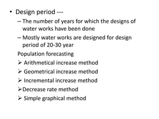
The document discusses several common methods for population forecasting used in urban planning and design of water works, including: - Arithmetical increase method which assumes a constant population increase over time, generally providing lower estimates. - Geometrical increase method which assumes a constant percentage increase, providing higher estimates as the percentage rarely remains constant. 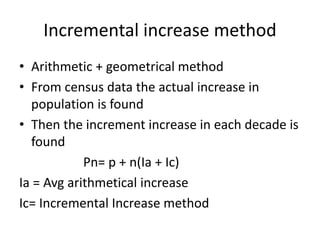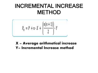- Incremental increase method which combines arithmetical and geometrical by using actual census data on population changes. - Decrease rate method which models decelerating growth approaching a saturation population based on practical constraints. - Graphical methods which plot past population data and extend trends to forecast future populations based on comparisons to other similar cities.

1. Design period

2. • Design period ---
– The number of years for which the designs of
water works have been done
– Mostly water works are designed for design
period of 20-30 year
Population forecasting
 Arithmetical increase method
 Geometrical increase method
 Incremental increase method
Decrease rate method
 Simple graphical method

3. Arithmetical increase method
• Simple method of population forecasting
• It generally gives lower results
• In this method increase in population from
decade to decade is kept constant
• This method is for large cities , which have
reached their saturation population

4. Formula
• Pn = p+nl
– Pn= population after n decades
– n = no of years in decades
– I = avg increment for a decade
n
year 2013 1989 1947
End year 2023 2004 2015
1 0.5 6.8

5. Year population ?
1931 12000
1941 16500
1951 26800
1961 41500
Increment per decade
-
4500
10300
14700

6. Geometrical increase method
• Percentage increase in population is kept
constant
• This method gives higher results , since %
increase never remains constant

7. Year population ?
1931 12000
1941 16500
1951 26800
1961 41500

8. Incremental increase method
• Arithmetic + geometrical method
• From census data the actual increase in
population is found
• Then the increment increase in each decade is
found
Pn= p + n(Ia + Ic)
Ia = Avg arithmetical increase
Ic= Incremental Increase method

9. Year population ?
1931 12000
1941 16500
1951 26800
1961 41500

10. year 1931 1941 1951 1961 1971 1981 1991
populati
on
12000 16500 26800 41500 57500 68000 74100

11. INCREMENTAL INCREASE
METHOD
X = Average arithmetical increase
Y= Incremental Increase method

12. Example:
• Predict the population for the year 2021, 2031,
and 2041 from the following population data
using the incremental increase method.
YEAR POPULATION
1961 860,741
1971 989,726
1981 1,201,897
1991 1,689,890
2001 2,079,270
2011 2,601,071

14. SOLUTION
For year 2021
For year 2031
For year 2041

15. Decrease rate method
• Decelerating growth is assumed to
asymptotically approach a saturation
population, that is, the maximum population
predicted for the geographic area of interest.
• The saturation population may be based on
practical limitations such as the maximum
number of dwellings under the zoning
restrictions or other constraints.

16. • As a rule, the larger a city becomes, the
smaller will be the rate of growth from year to
year
• The Saturation population must be estimated.
Note: the saturation population is the maximum
number of people can inhabit a town based on
the physical constraints of buildable land
zoning.

17. Formula
dp/dt= Kd(S-P)
Kd = P= P1 + (S-P1)(1-e-Kd (t - t
1
) )
P = population
t = time
Kd = decreasing rate of increase growth constant
S = Saturation population

18. Year population Increase Percentage
increase in
population
Decrease in %
increase
1940 8000
1950 12000
1960 17000
1970 22500
Total
Average
Year Net % increase
in population
population
1980 32.4-8.8=23.6 22,500 + (23.6/100)*22,500 =27,810
1990
2000

19. GRAPHICAL METHOD

20. SIMPLE GRAPHICAL METHOD
• In this method, the populations of last few
decades are correctly plotted to a suitable
scale on graph
• This extension should be done carefully and it
requires proper experience and judgment.
• The best way of applying this method is to
extend the curve by comparing with
population curve of some other similar cities
having the similar growth condition.

22. COMPARATIVE GRAPHICAL METHOD
• In this method the census populations of cities
already developed under similar conditions
are plotted.
• The curve of past population of the city under
consideration is plotted on the same graph.
• The curve is extended carefully by comparing
with the population curve of some similar
cities having the similar condition of growth
• The advantage of this method is that the
future population can be predicted from the
present population even in the absence of
some of the past census report.

29. MASTER PLAN METHOD
• The big and metropolitan cities are generally not
developed in haphazard manner, but are planned and
regulated by local bodies according to master plan.
• According to the master plan the city is divided into
various zones such as residence, commerce and industry.
• The population densities are fixed for various zones in
the master plan.
• From this population density total water demand and
wastewater generation for that zone can be worked out.
• By this method it is very easy to access precisely the
design population.

30. Logistical curve method
• This method is used when the growth rate of
population due to births, deaths and
migrations takes place under normal situation
and it is not subjected to any extraordinary
changes like epidemic, war, earth quake or any
natural disaster, etc.,
• and the population follows the growth curve
characteristics of living things within limited
space and economic opportunity

31. Logistical curve method
• If the population of a city is plotted with respect to
time, the curve so obtained under normal condition
looks like S-shaped curve and is known as logistic curve

32. Formula
• Equation of the logistic curve
Ps= Saturation population

33. Saturation population Ps
P0 , P 1 , P2 = Population of the city at the time t0 , t2 , t3

34. Problem
The population of a city in three consecutive
years i.e. 1991, 2001 and 2011 is 80,000;
250,000 and 480,000, respectively. Determine
(a) The saturation population, (b) The
equation of logistic curve, (c) The expected
population in 2021.

35. Solution
• P0 = t0 =
• P1 = t1 =
• P0 = t2 =