This document introduces the concept of the derivative and rate of change in mathematics. It defines the derivative as the slope of the tangent line to a curve at a point, which can be interpreted as the instantaneous rate of change of the dependent variable with respect to the independent variable. The document provides examples of calculating derivatives and interpreting them in the context of rates of change. It then discusses how to view the derivative not just at a single point, but as a new function defined for all points where the limit exists, known as the derivative function.

1. 2.7
Derivatives and Rates
of Change

2. 2
Derivatives and Rates of Change
The problem of finding the tangent line to a curve
involve finding a limit.
This special type of limit is called a derivative and
we will see that it can be interpreted as a rate of
change in any of the natural or social sciences or
engineering.

3. 3
Tangents

4. 4
Tangents
If a curve C has equation y = f(x) and we want to find the
tangent line to C at the point P(a, f(a)), then we consider a
nearby point Q(x, f(x)), where x  a, and compute the slope
of the secant line PQ:
Then we let Q approach P along the curve C by letting
x approach a.

5. 5
Tangents
If mPQ approaches a number m, then we define the tangent
t to be the line through P with slope m. (This amounts to
saying that the tangent line is the limiting position of the
secant line PQ as Q approaches P. See Figure 1.)
Figure 1

6. 6
Tangents

7. 7
Example 1
Find an equation of the tangent line to the parabola y = x2
at the point P(1, 1).
Solution:
Here we have a = 1 and f(x) = x2, so the slope is

8. 8
Example 1 – Solution
=
= 1 + 1
= 2
Using the point-slope form of the equation of a line, we find
that an equation of the tangent line at (1, 1) is
y – 1 = 2(x – 1) or y = 2x – 1
cont’d

9. 9
Tangents
If h = x – a, then x = a + h and so the slope of the secant
line PQ is
(See Figure 3 where the case h > 0 is illustrated and Q is to
the right of P. If it happened that h < 0, however, Q would
be to the left of P.)
Figure 3

10. 10
Tangents
Notice that as x approaches a, h approaches 0 (because
h = x – a) and so the expression for the slope of the
tangent line in Definition 1 becomes

11. 11
Derivatives

12. 12
Derivatives
We have seen that the same type of limit arises in finding
the slope of a tangent line (Equation 2)
In fact, limits of the form
arise whenever we calculate a rate of change in any of the
sciences or engineering, such as a rate of reaction in
chemistry or a marginal cost in economics.
Since this type of limit occurs so widely, it is given a special
name and notation.

13. 13
Derivatives
If we write x = a + h, then we have h = x – a and h
approaches 0 if and only if x approaches a. Therefore an
equivalent way of stating the definition of the derivative, as
we saw in finding tangent lines, is

14. 14
Example 4
Find the derivative of the function f(x) = x2 – 8x + 9 at the
number a.
Solution:
From Definition 4 we have

15. 15
Example 4 – Solution cont’d

16. 16
Derivatives
We defined the tangent line to the curve y = f(x) at the point
P(a, f(a)) to be the line that passes through P and has
slope m given by Equation 2 .
Since, by Definition 4, this is the same as the derivative
f(a), we can now say the following.

17. 17
Derivatives
If we use the point-slope form of the equation of a line, we
can write an equation of the tangent line to the curve
y = f(x) at the point (a, f(a)):
y – f(a) = f(a)(x – a)

18. 18
Rates of Change

19. 19
Rates of Change
Suppose y is a quantity that depends on another quantity x.
Thus y is a function of x and we write y = f(x).
If x changes from x1 to x2, then the change in x (also called
the increment of x) is
x = x2 – x1
and the corresponding change in y is
y = f(x2) – f(x1)

20. 20
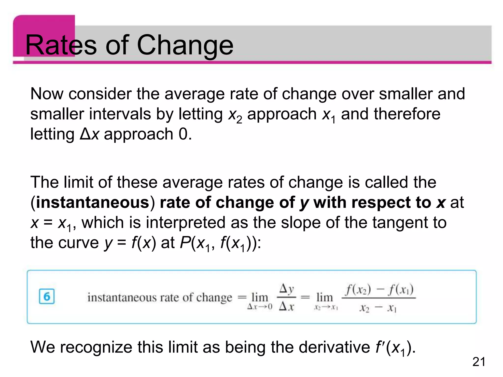
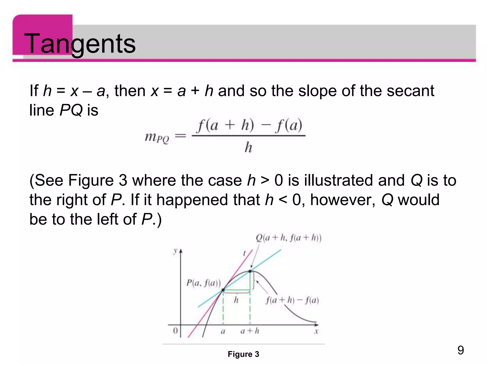
Rates of Change
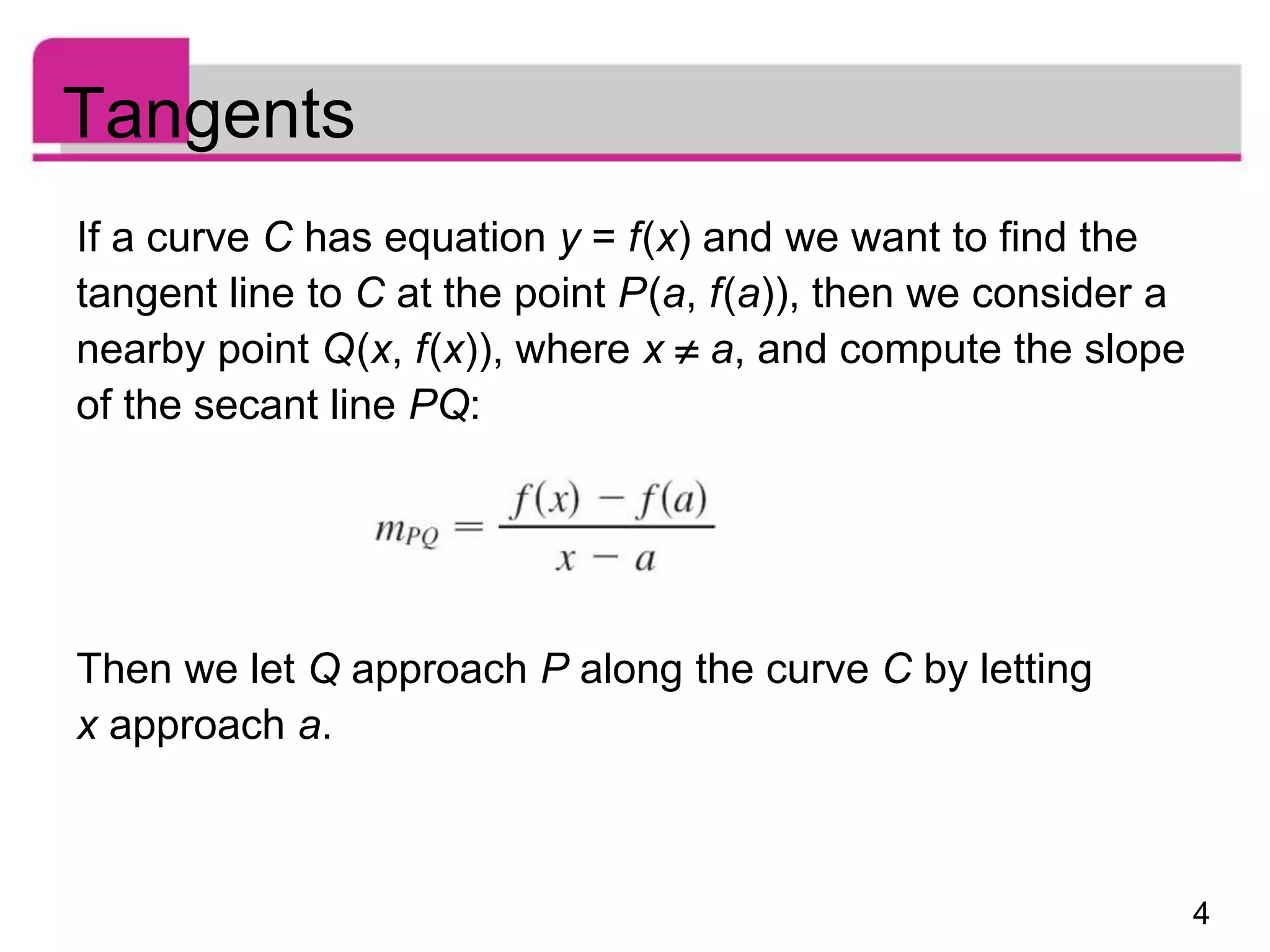
The difference quotient
is called the average rate of
change of y with respect to x
over the interval [x1, x2] and
can be interpreted as the slope
of the secant line PQ
in Figure 8.
Figure 8
average rate of change = mPQ
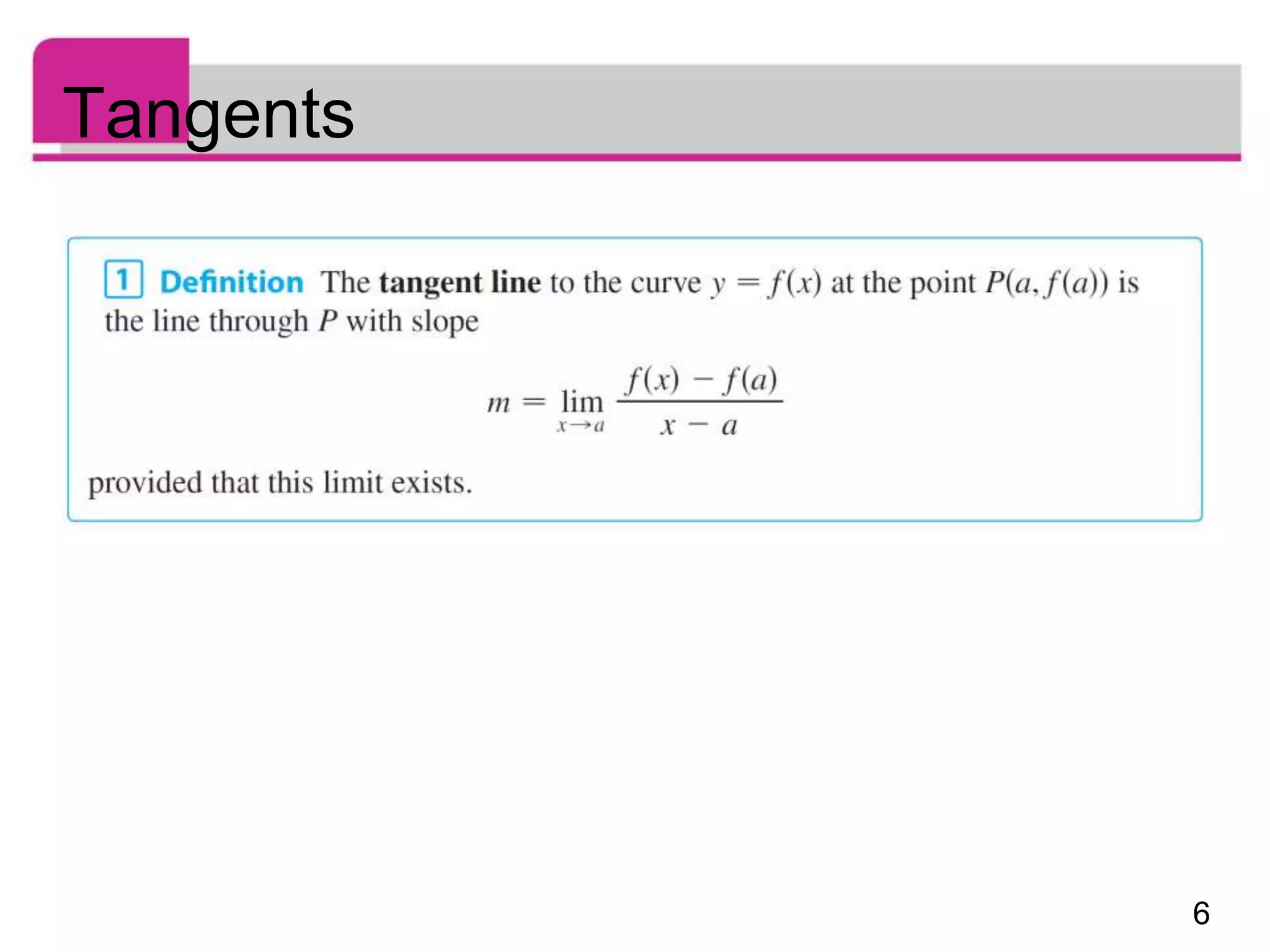
instantaneous rate of change =
slope of tangent at P

21. 21
Rates of Change
Now consider the average rate of change over smaller and
smaller intervals by letting x2 approach x1 and therefore
letting Δx approach 0.
The limit of these average rates of change is called the
(instantaneous) rate of change of y with respect to x at
x = x1, which is interpreted as the slope of the tangent to
the curve y = f(x) at P(x1, f(x1)):
We recognize this limit as being the derivative f(x1).

22. 22
Rates of Change
We know that one interpretation of the derivative f(a) is as
the slope of the tangent line to the curve y = f(x) when
x = a. We now have a second interpretation:
The connection with the first interpretation is that if we
sketch the curve y = f(x), then the instantaneous rate of
change is the slope of the tangent to this curve at the point
where x = a.

23. 23
Example 6
A manufacturer produces bolts (one bolt represents a strip
of cloth 100 yards) of a fabric with a fixed width. The cost
of producing x yards of this fabric is
C = f(x) dollars.
(a) What is the meaning of the derivative f(x)? What are its
units?
(b) In practical terms, what does it mean to say that
f(1000) = 9?
(c) Which do you think is greater, f(50) or f(500)?
What about f(5000)?

24. 24
Example 6(a) – Solution
The derivative f(x) is the instantaneous rate of change of C
with respect to x; that is, f(x) means the rate of change of
the production cost with respect to the number of yards
produced.
Because
the units for f(x) are the same as the units for the
difference quotient C/x.
Since C is measured in dollars and x in yards, it follows
that the units for f(x) are dollars per yard.

25. 25
Example 6(b) – Solution
The statement that f(1000) = 9 means that, after 1000
yards of fabric have been manufactured, the rate at which
the production cost is increasing is $9/yard.
(When x = 1000, C is increasing 9 times as fast as x.)
Since x = 1 is small compared with x = 1000, we could
use the approximation
and say that the cost of manufacturing the 1000th yard
(or the 1001st) is about $9.
cont’d

26. 26
Example 6(c) – Solution
The rate at which the production cost is increasing
(per yard) is probably lower when x = 500 than when x = 50
(the cost of making the 500th yard is less than the cost of
the 50th yard) because of economies of scale. (The
manufacturer makes more efficient use of the fixed costs of
production.)
So
f(50) > f(500)
cont’d

27. 27
Example 6(c) – Solution
But, as production expands, the resulting large-scale
operation might become inefficient and there might be
overtime costs.
Thus it is possible that the rate of increase of costs will
eventually start to rise.
So it may happen that
f(5000) > f(500)
cont’d

28. 28
2.8 The Derivative as a Function

29. 29
We have considered the derivative of a function f at a fixed
number a:
Here we change our point of view and let the number a
vary. If we replace a in Equation 1 by a variable x, we
obtain
The Derivative as a Function

30. 30
The Derivative as a Function
Given any number x for which this limit exists, we assign
to x the number f′(x). So we can regard f′ as a new function,
called the derivative of f and defined by Equation 2.
We know that the value of f′ at x, f′(x), can be interpreted
geometrically as the slope of the tangent line to the graph
of f at the point (x, f(x)).
The function f′ is called the derivative of f because it has
been “derived” from f by the limiting operation in Equation 2.
The domain of f′ is the set {x|f′(x) exists} and may be
smaller than the domain of f.